Course:CPSC522/Reinforcement Learning with Function approximation

Reinforcement Learning with Function Approximation

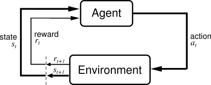
Reinforcement Learning is an area of machine learning inspired by behaviorist psychology, concerned with how software agents ought to take actions in an environment so as to maximize some notion of cumulative reward. For smaller problems machine learners use a tabular representation of the data called a Look-up Table (LUT) in order to make the decisions leading to a maximal reward. Here we are introducing a new method called Reinforcement Learning with Function Approximation to overcome issues with LUTs such as limited memory and how they are impractical when dealing with huge data.^[1]

Principal Author: Mehrdad Ghomi
Collaborators: Jiahong Chen, Jordon Johnson

Abstract

If we assume that our estimates of value functions are represented as a table with one entry for each state or for each state-action pair, then we have a particularly clear and instructive case; but it is limited to tasks with small numbers of states and actions. The problem is not just the memory needed for large tables, but the time and data needed to fill them accurately. In other words, the key issue is that of generalization. This is a severe problem. In many tasks to which we would like to apply reinforcement learning, most states encountered will never have been experienced exactly before. This will almost always be the case when the state or action spaces include continuous variables or complex sensations, such as a visual image. The only way to learn anything at all on these tasks is to generalize from previously experienced states to ones that have never been seen. Fortunately, generalization from examples has already been extensively studied, and we do not need to invent totally new methods for use in reinforcement learning. To a large extent we need only combine reinforcement learning methods with existing generalization methods. The kind of generalization we require is often called function approximation because it takes examples from a desired function (e.g., a value function) and attempts to generalize from them to construct an approximation of the entire function. ^[1]

Builds on

Function approximation is an instance of supervised learning (a primary topic studied in machine learning), artificial neural networks, pattern recognition, and statistical curve fitting. In principle, any of the methods studied in these fields can be used in reinforcement learning.

More general than

Function approximation is used to replace inefficient and impractical Look-up Tables. We can also use neural networks to replace the LUTs and approximate the Q-function in Q-Learning, a model-free reinforcement learning technique in which optimal action-selection of a policy for any given finite Markov Decision Process (MDP) will be learned.
Later on we will develop a method called Reinforcement Learning with Back Propagation, which will build on RL with Function Approximation.^[2] For a very cool applet for playing and working with Q-Learning click here^[6]

Content

There are traditionally two different learning paradigms: unsupervised learning and supervised learning. Reinforcement Learning (RL) can be introduced as a third learning paradigm. RL is characterized as learning that takes place via interaction of a learning agent with its environment. Like supervised learning, a feedback signal is required; however, for RL this feedback signal represents a reward, not a desired value. RL is therefore not supervised learning. The purpose of RL is to learn which actions yield the greatest reward.^[2]

Elements of RL

Policy

In RL, the policy (denoted by the symbol π) defines a learning agent's way of behaving at any given time. It is a function of the rules of the environment, the current learned state and how the agent wishes to select future states or actions. It provides a mapping from perceived states to actions to be taken. An optimal policy is one which accumulates the greatest rewards over the specified term. The policy is in effect realised by the value function that is being learned using RL and changes as the value function is being learned. You may come across the terms “on-policy” & “off-policy”. The difference is simply that on-policy is both learning and using (to control actions) the same policy that is being learned. “Off-policy” methods learn one policy, while using another to decide what actions to take while learning.^[2]

Reward Function

A reward function defines the goal. Given any state of the environment, the reward function identifies how good or bad this state (or a given action while in this state) is.^[2]

Value Function

The difference between a value function and a reward function is subtle. Whereas the reward function measures the reward associated with the immediate state of the system, a value function represents a prediction of reward at some future time, based on the current state. It takes into account all future rewards that may ensue as a result of reaching the current state.^[2]

$V(s_{t})=r_{t}+\gamma V(s_{t+1})$

$V(s_{t})=r_{t}+\gamma r_{t+1}+\gamma ^{2}r_{t+2}+...+\gamma ^{t_{n}}r_{T}$

Model(optional)

In RL, a model is typically the set of probability functions that determine how an agent would behave in any given state of the system. While it is a requirement for some types of RL (e.g. Dynamic Programming), it is not necessary for the type of learning that will be addressed in this course. ^[2]

Example

Tic-Tac-Toe

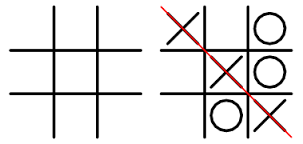
Tic-Tac-Toeor “Noughts-and-Crosses” is a simple game played on a 3x3 grid. The objective is to be the first to make a line of crosses or noughts across the grid. The environment in this case, is the board. The reward function is simple, but can only be defined for the final state to indicate a win, a loss or a draw. Given that the environment of all possible states is small and reasonably manageable, the value function can be implemented as a table indexed by all possible states. (One may even wish to take advantage of the symmetrical nature of the board and reduce the number of actual states referenced in this table). The policy takes into account the rules of the game and its choices are dictated by all possible states that it can select given its current state. The effect of RL is to learn a value function that can reliably predict if a state (the next move) will result in a win or not. If a loss and draw are considered to be equal, then the terminal states in the table that represents the value function can be set to 1 or 0. All others would be initialized to 0.5 (i.e. probability of a win is known to be no better than chance).Tic-tac-toe has a small finite number of states and the value function can be implemented as a look-up table. In the above figure, each separate board position has an associated probability. As play proceeds, the computer will perform a search of all possible moves and select that move for which the value function indicates the greatest likelihood of winning. Given that the value function will return 0.5 for all initial states, the earliest games in the learning process will be unlikely to win against an intelligent player. Most moves will be greedy moves, i.e. selection of a move that has the highest value. However it is useful at times to select moves randomly. These moves, although not necessarily the best, are termed exploratory moves as they help to experience states that would otherwise not be encountered. During play, the learning process updates the entries in the table, attempting to improve their accuracy. Over time and after playing many games, the value function will return values that represent the true probabilities of winning from each state.^[2]

Motivation (Look-up Table Versus Function Approximation)

Although current Reinforcement Learning methods have shown some good successes in some application domains, we still need to address several important theoretical issues before having a fully competent and versatile learning method. One important challenge is dealing with problems with large or continuous state/action spaces. In these problems, the look-up table approach is not feasible anymore since there is no way to enumerate all values (there are an infinite number of then). Function approximation (FA) techniques should come at rescue, but our understanding of the interplay between function approximation and RL methods is limited in a number of important ways. In the early stages of RL research, there were many examples and counter-examples that show the feasibility or the infeasibility of using FA in RL. Gradually, the theory started to develop, and the conditions and situations that FA can be used in a RL setting were revealed. However, this problem has not been solved completely and researchers still need to work on it, to create methods that work more efficiently for a larger class of problems. ^[9]

Function Approximation

Optimal and Approximate Value Function When we start learning, the value function is typically randomly initialized:

$V(s_{t})$

It will be a poor approximation to what we actually want, which is the optimal value function denoted as follows:

$V^{*}(s_{t})$

This is the value function that will lead to us making the best decisions. By best, we mean the best or most reward possible. Thus the approximate value at some state $s_{t}$ is equal to the true value at that state, plus some error in the approximation. We could write this as follows:

$V(s_{t})=e(s_{t})+V^{*}(s_{t})$ ^[2]

One thing that needs to be clear and understood is that when using approximation, convergence is no longer guaranteed. The reason is that using the neural Network at each iteration of training we approximate the value-function by changing the weights of the network. In this case we have infinite number of state-action members for which we don’t know exactly the Q-values. We just use weights and biases of the network, which are obtained by training the network using a finite number of discrete (quantized) state-action spaces from the LUT, to approximate the Q-values.

Bellman Equation

Richard Bellman (1957) defined the relationship between a current state and its successor state. It is often applied to optimization problems that fall in a branch of mathematics known as dynamic programming.

$V(s_{t})=r_{t}+\gamma V(s_{t+1})$

The equation is recursive in nature and suggests that the values of successive states are related. In RL, the Bellman equation computes the total expected reward. Typically we want to follow a sequence of events (a policy) that generate the maximum rewards (the optimal policy). Here we introduce two new terms. The immediate reward r and the discount factor γ. ^[2]

Convergence Rate

Let the error in the value function at any given state be represented by:

$e(s_{t})$

Then:

$V(s_{t})=e(s_{t})+V^{*}(s_{t})$

and:

$V(s_{t+1})=e(s_{t+1})+V^{*}(s_{t+1})$

Using the Bellman equation:

$V(s_{t})=r_{t}+\gamma V(s_{t+1})$

we can derive that:

$e(s_{t})=\gamma e(s_{t+1})$

Concluding that the error in successive states is related. But we know that already, since we know that the future rewards V(s) are themselves are related. However, the interesting thing is that we can show that these rewards actually converge. I.e. after enough training no longer causes them to change. For a decision process where a reward is available at a terminal state, we know that the reward is known precisely. I.e. there is no error in the reinforcement signal. Given:

$e(s_{t})=\gamma e(s_{t+1})$

we deduce that with enough sweeps through the state space, I.e. enough opportunities to learn, we will eventually reach the condition where e(s) is zero for all t. When this is the case, then we know we have the optimal value function.

$V(s_{t})=e(s_{t})+V^{*}(s_{t})$

For the optimal value function, we can say that we have state values that satisfy the Bellman equation, for all t: ^[2]

$V(s_{t})=r+\gamma V(s_{t+1})$

Q-Learning

Q-learning is a model-free reinforcement learning technique. Specifically, Q-learning can be used to find an optimal action-selection policy for any given (finite) Markov decision process (MDP). It works by learning an action-value function that ultimately gives the expected utility of taking a given action in a given state and following the optimal policy thereafter. A policy is a rule that the agent follows in selecting actions, given the state it is in. When such an action-value function is learned, the optimal policy can be constructed by simply selecting the action with the highest value in each state. One of the strengths of Q-learning is that it is able to compare the expected utility of the available actions without requiring a model of the environment. Additionally, Q-learning can handle problems with stochastic transitions and rewards, without requiring any adaptations. It has been proven that for any finite MDP, Q-learning eventually finds an optimal policy, in the sense that the expected value of the total reward return over all successive steps, starting from the current state, is the maximum achievable.

SARSA

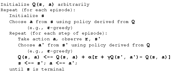
The Sarsa algorithm is an On-Policy algorithm for TD-Learning. The major difference between it and Q-Learning, is that the maximum reward for the next state is not necessarily used for updating the Q-values. Instead, a new action, and therefore reward, is selected using the same policy that determined the original action. The name Sarsa actually comes from the fact that the updates are done using the quintuple Q(s, a, r, s', a'). Where: s, a are the original state and action, r is the reward observed in the following state and s', a' are the new state-action pair. The procedural form of Sarsa algorithm is comparable to that of Q-Learning:

Generalization

Reinforcement learning systems must be capable of generalization if they are to be applicable to artificial intelligence or to large engineering applications. To achieve this, any of a broad range of existing methods for supervised-learning function approximation can be used simply by treating each backup as a training example. Gradient-descent methods, in particular, allow a natural extension to function approximation of all the techniques developed in other related areas, including eligibility traces. Linear gradient-descent methods are particularly appealing theoretically and work well in practice when provided with appropriate features. Choosing the features is one of the most important ways of adding prior domain knowledge to reinforcement learning systems. Linear methods include radial basis functions, tile coding, and Kanerva coding. Backpropagation methods for multilayer neural networks are methods for nonlinear gradient-descent function approximation.^[1]

Generalization with Multi-Layer Perceptrons (Neural Network)

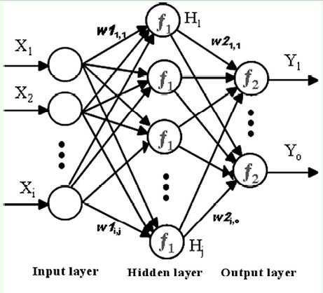
For instructional purposes, the implementation of RL is by far the easiest using look-up tables. Each value or Q-value is indexed by the states of the problem. Initially randomly initialized, as each state is visited, and gets updated. However, as the number of states increases so does the size of the look up table and the number of computations to adequately populate it. In practice, with a world with many dimensions, the number of states will be large. 1020 states for a Back-Gammon game, not only is memory a concern, but more so generalization. A sparsely populated table is unlikely to be effective. The answer is to generalize the value functions. There are many approaches including the application of non-linear approximators such as mutli-layer perceptrons. However, the area is still one of active research. In fact the application of neural nets, although promising and shown to be highly successful in Back-Gammon is regarded as a delicate art! Two approaches to the practical assignment are suggested. Both require the use of a neural network (multi-layer perceptron) trained using the Backpropagation algorithm. Note there are issues with both approaches suggested below: ^[2,3]

Online training

The Q-function is implemented as an MLP. As Temporal Difference(TD) updates are backed up, the supervised values for the Backpropagation training targets are generated according to TD as applied to the Q-function. Thus the MLP is undergoing training as it is being used.

Offline training

The Q-function is implemented as a look-up table during training. As TD updates are backed up, the table is updated. Upon completion of RL training, the contents of the look-up table are then used to train a neural net. Once trained, the neural net is used to replace the look-up table in the RL agent. We then observe improvements in the agent’s behavior now using a generalized Q-function.
For playing and working with a very useful tool for Neural Networks click here.^[4] For playing and working with a very useful tool for Multi-Layer Perceptron click here.^[5] For Java implementation of different types of Neural Nets click here^[7]

When RL Fails

While RL and in particular temporal difference learning, seems generally suitable for learning many varieties of control problems, in order to do so, a learning agent requires interaction with its environment. In certain cases this might not be desirable or possible.
For example, learning to fly an airplane. You would not let an untrained agent take control of a real aircraft. Either some software would be necessary to restrict the agents actions to “safe” actions or possibly, to train it first using a simulator. (An approach which works well with real pilots).
How about applying RL in the health/medical realm? RL might be able to provide personalized care by learning to adjust medications on an individual basis. For example in anesthesiology, where the delivery of anesthetic is carefully governed based upon monitoring a patients vital signs. However again, the application of RL is unacceptable because initially, the agent will require exploration before it can learn to offer optimal dosing. Unlike training a pilot, in this case there is no simulator available for pre-training. With regards to this, one solution from the literature is to adopt an approach which attempts to off-line learn from collected data.^[8]

Annotated Bibliography

[1] Richard S. Sutton and Andrew G. Barto (1998). Reinforcement Learning: An Introduction. The MIT Press. ISBN 0262193981, 9780262193986 Reinforcement Learning: An Introduction (HTML format)
[2] UBC ECE 592 Course - Instructed by: Dr. Sarbjit Sakaria ECE 592- Architecture Design for Learning Systems
[3] Recurrent Neural Network Based Approach for Solving Groundwater Hydrology Problems: Ivan N. da Silva, José Ângelo Cagnon and Nilton José Saggioro - ISBN 978-953-51-0935-8, Published: January 16, 2013 under CC BY 3.0 license.
[4] David Poole, Alan Macworth. AISpace.org - Copyright © 1999 - 2010
[5] The OCHRE applet (Optical CHaracter REcognition)
[6] Dr. Ir. Frank Vander Berghen - Kranf Site - Q-learning Crawling Robot applet
[7] Neuroph Java Neural Network Framework - Zoran Sevarak.
[8] Neural Fitted Q Iteration - First Experiences with a Data Efficient Neural Reinforcement Learning Method, Martin Riedmiller, Neuroinformatics Group, University of Onsabru ̈ck, 49078 Osnabruck
[9] Reinforcement Learning and Artificial Intelligence (RLAI) - University of Alberta - RLFA Webpage

To Add

Fun tool for Q-Learning
Reinforcement Learning for Cellular Telephones
Backpropagation for Image Compression
Cat and Mouse Game Reinforcement Learning