Course:CPSC522/Markov Decision Process

Markov Decision Process

A Markov Decision Process(MDP) is a mathematical framework for modeling decision making; mostly when the agent needs to go beyond a set of fixed decisions or where the outcomes are partly random and it is not clear how long the agent has to keep going.

Principal Author:Md Abed Rahman
Collaborators:Yaashaar Hadadian Pour , Adnan Reza

Abstract

This page tries to present some insight into Markov Decision Processes(MDP): what are they, why are they used, implementation level ideas and existing extensions.

Markov Decision Processes are essentially markov chains that are augmented with actions and rewards. They are useful to model situations with infinite or indefinite horizons , i.e. the agent is not sure when the process might stop. Due to this uncertainty of the system, the agent running a MDP usually work based on feedbacks(called rewards) that the agent receives by performing an action. These rewards can be said to dictate an agents policy in many ways. This interesting property can be attributed to the fact that the notion of utility is not present here, since there is no guarantee on halting. After reaching a terminal state, the agent stops. MDPs are of particular interest as they are particularly useful when it comes to formalizing a bunch of optimization problems and these notions could also be extended to study reinforcement learning. Again, we will focus on the inner workings of an MDP and also briefly go through some well known extensions.

Builds on

This concept builds on Decision Networks which are applicable for domains that are partially observable and have a finite horizon, i.e. the process is known to end at a certain time. But since, MDPs deal with problems which are not guaranteed to halt at a given time(or not at all at times), the concept of utility does not strictly hold anymore.

Related Pages

As mentioned before, MDPs build on decision networks. All of these originate from the concept of bayesian networks which are used to model uncertainty in the environment.

Content

Definition

Markov Decision Process

We define a MDP as a 4-tuple $(S,A,P(S_{t+1}|S_{t},A_{t}),R(s,a,s')$ , where

• $S$ is a finite set of states,
• $A$ is a finite set of actions (alternatively, $A_{s}$ is the finite set of actions available from state $s$),
• $P(S_{t+1}|S_{t},A_{t})$ is the transition model,
• $R(s,a,s')$ is the immediate reward (or expected immediate reward) received after moving to state $s'$ from state $s$ by performing action $a$

Lets take a look at the individual elements of the 4-tuple that defines a MDP. $S$ can simply be interpreted as the set of the different number of configurations the system can go through. Based on the context of the problem it can be quite varied. For example, if an MDP is used to solve a problem where in the salmon harvesting season the agent has to make decisions on how much salmon to catch given the approximate salmon population of the river and how much to leave in order to let them reproduce; a state would be the a number/metric that signifies the salmon population at a given time. Here, $S$ is the number of all such states.
As mentioned before, $A$ is the set of actions. In our salmon harvesting problem example, the number of fishes to catch at a given time would be an action. The set of all such actions makes the set $A$ for this given problem.
From this same context, the term $P(S_{t+1}|S_{t},A_{t})$ would be the transition model that specifies the change is the population from year $t$ to year $t+1$
Finally, $R(s,a,s')$ in this context could be the revenue achieved or some measure that signifies how well the salmon population has been preserved. It can also be a mixture of both.

MDP Problem Definition

The problem associated with MDPs is defined as finding a "policy" for the decision maker (i.e. the agent). A policy is the expression of what the agent should do at a certain state to get the most favorable outcome as the decision process unfolds. A policy for an MDP is a single decision function $\pi (s)$ that specifies what the agent should do for each state. Once the policy is defined for an MDP, action to be taken for each state is fixed and the resulting combination behaves like a Markov chain. The agent usually starts in a initial state dubbed as the start state, selects an action, ends up in another state, selects another action and so on. The motivation that drives a policy is the reward or punishment(positive or negative feedback) defined for each action, given the agent is at a certain state. The goal is to choose a policy $\pi$ that will maximize some cumulative function of the random rewards, i.e. maximizes the expected utility or reward of a policy $\pi (s)$ It can be shown by the expression: $\sum _{t=0}^{\infty }{P(s_{0},s_{1},....,s_{term})\times R(s_{0},s_{1},....,s_{term})}$    (where we choose $a_{t}=\pi (s_{t})$)
Here, $a_{t}=\pi (s_{t})$ means the action prescribed by policy $\pi$ when the agent is at state $s_{t}$
For our salmon harvest problem, a policy would dictate the amount of fish to be harvested that gives the highest expected reward. In this case, the reward could be the optimized amount of revenue with a high value for a measure that signifies how well the salmon population has been preserved.

Reward and Optimal Policy

Based on how the rewards/ penalties are defined for an agent, the optimal policy changes. The agent always tries going to states that maximizes rewards and based on how the rewards are set, the agent also tries to maximize expected rewards. We can look at the following toy example for a better understanding.
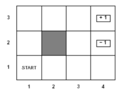
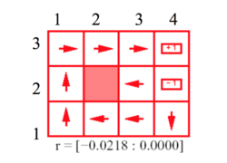
In our toy example, we have this grid world with 3 rows and 4 columns. A state is defined as the coordinate value of where the agent is at a given time instance. To define the coordinate of a certain cell we go first in the x direction and then in the y direction. So, the state marked 'Start'(coordinate (1,1)) is the start state. When the agent moves to one of the cells marked (4,2) or (4,3), the execution comes to a halt. We call (4,2) and (4,3) to be the terminal states of the given system. State (2,2) is unreachable and the grid world is surrounded by walls. Based on which state the agent is in(given the state is a non terminal state), the policy will change.The agent can only go up,down,left and right, moving one block at a time. Here, it is important to note, even if the optimal policy dictates moving to a certain state, the agent might end up in other states with some probability. Basically, due to the stochastic nature of the system, an MDP is not exactly like a finite state machine; where actions lead to deterministic transitions.For example, in our grid world, when the agent makes an attempt to move in a certain direction, it succeeds with probability 0.8. It might also make an unsuccessful move to any one of its adjacent steps based on the direction the move is attempted with probability 0.1. Based on how an agent is rewarded or punished for making a move to a state other than one of the terminal states[rewards for each of the terminal state are considered to be constants in this case] the optimal policy will change as the agent would act differently based on how rewards for a certain action is defined as.Again, the agent knows its start state and the rewards/punishment associated with reaching any of the terminal states. Now, as we mentioned before, how the agent is punished/rewarded for being in a certain state can change the policy of the agent. We must remember, our agents primary objective is not to reach a terminal state with positive rewards[In this case it's (4,3)], but to maximize it's expected rewards if and when it reaches it. This results in rewards achieved from transitioning into intermediary steps having an influence on the optimal policy. The following pictures show how various reward/penalty values for traversing the grid can have an effect on the optimal policy:

• 

  The Grid World

• 

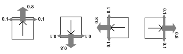  Possible moves with probabilities

• 

  1

• 

  2

• 

  3

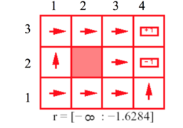
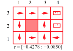
The pictures above show the actions that are dictated by the optimal policy, given the agent is at a certain state. The arrows indicate which way the agent will try to move when it is at a certain stage, a move which is prescribed by the optimal policy. The r values given under each figure shows the positive or negative rewards(i.e. punishment) received from reaching a state other than the terminal states. These examples illustrate how optimal policy is guided by rewards/punishments of reaching a certain state. In the first picture, we can see that the penalty is high for exploration[r<-1.6284]. In cases like this, the agent makes sort of a kamikaze charge to the nearest terminal state regardless of the reward/punishment received. This behavior is due to the fact that exploration was more costly than the reward/ punishment received from reaching one of the terminal states. Thus the optimal policy was to reach one of the terminal states as it was better to reach a terminal state with negative rewards than to roam around through the grid. In the second picture, the penalty of transitioning into a non terminal state is not as much as before [-0.4278<r<-0.0850], but the cumulative punishment for staying in the grid is still pretty big. As we can guess, this time, the agent will try not to hang around in the grid but try to reach the terminal state. However, in contrast to the example before, this time the agent will no longer make a kamikaze charge to any one of the terminal states and try to reach a terminal stage with positive rewards. The interesting part of the optimal policy would be the part where the agent finds itself in one of the states in the set {(2,1),(2,2),(2,3)}. When the agent is in one of these states, taking a path that makes sure that the agent can somehow avoid the punishing terminal state (4,2) is not an option, because in that case, the cumulative punishment for staying in the grid longer overshoots the reward achieved from reaching the rewarding terminal state (4,3). Thus, the optimal policy consists of going through (3,2) to reach (4,3) though there is a chance of slipping into (4,2). For the 3rd picture where exploration is cheaper[-0.0218<r<-0.000], the agent tries to move to the rewarding terminating state at (4,3) and also go away from the terminating state (4,2). This behavior is mostly noticeable when the agent is in the state (3,2). Since, it is better to roam than to reach (4,2); the agent will try to move towards (2,2), a stage it cannot reach. This policy takes advantage of the fact that even if it stays in it's position, there is a chance that it might slip in to either (3,3) or (3,1) with probability 0.1 each. Trying to go away from (4,2) instead of making a move towards(4,3), the agent makes sure that it never reaches (4,2) as now it has the option to move around a bit.
As mentioned before, rewards and optimal policy go hand to hand. A fun applet to play around with an examples similar to the ones mentioned above can be found here

Solution Approaches and Algortihms

Various solution approaches have been tried and proposed over the years, most of them being based on the concepts of dynamic programming or linear programming. Some popular algorithms are are brute force approach, value iteration, policy iteration. Before we take a look into these algorithms, we define some notation the algorithms use to find the optimal policy:

$V^{\pi }(s)$ the expected value of following policy $\pi$ in state $s$
$Q^{\pi }(s,a)$, where $a$ is an action: expected value of performing $a$ in $s$, and then following policy $\pi$. There is also notation for showing the reward. A reward can be discounted or total(i.e. additive). The whole discounted reward is as follows:
$V=r_{1}+\gamma ^{2}r_{2}+\gamma r_{3}+.....$
Where $\gamma$ is the discount factor $0\leq \gamma \leq 1$. The reason of keeping this discount factor would be to make sure that the total value is finite, thus making this expression is appropriate for infinite domain problems.
Then we get the following bellman equation for $Q$ :
$Q^{\pi }(s,a)=\sum _{s'}{P(s'|s,a)\times (R(s,a,s')}+\gamma V^{\pi }(s'))$    
As mentioned before, $R(s,a,s')$ is the reward of moving to state $s'$ from $s$ by performing action $a$ . This means that, if the agent is in state $s$, performs action $a$, and arrives in state $s'$, it gets the immediate reward of $R(s,a,s')$ plus the discounted future reward, $\gamma$$V^{\pi }(s')$. As, the agent does not know the actual resulting state using the expected value makes sense.
Also, for the optimal policy we define the following:
$Q^{*}(s,a)$: Expected value of performing a in s, and then following the optimal policy $\pi ^{*}$.
$V^{*}(s)$: the expected value of following optimal policy $\pi ^{*}$ in state s

Now, we take a look at Brute force, Value Iteration and Policy Iteration here:

Brute Force Approach

If we take a brute force approach to solve an MDP then we go on to considering a simple enumeration algorithm.To do so, we look at the finite space of solutions: since there are a total of $|A|$ actions that can be returned for each state, there are a total of $|S|^{|A|}$ possible policies. This leads us to a simple algorithm: enumerate and evaluate all policies $\pi$ in a brute-force manner and return the best policy $\pi ^{*}$. As the solution space is exponential, this is not feasible. However, this gives us insights on how this becomes a dynamic programming problem which we will explore next.

Value Iteration

As mentioned before, value iteration or backward induction is essentially a dynamic programming approach. Value iteration finds better policies by construction i.e. finding the best value function by iteratively updating the value function. Value iteration starts with an arbitrary guess $V_{0}$ and uses the equations mentioned previously to get $V_{k+1}$. Defining a stopping condition is a bit tricky in Value Iteration. There are two approaches that can be used. Firstly, a certain number of steps $K$ is chosen as the number of times the algorithm will iterate. This number $K$ can be chosen by an expression based on the convergence of the algorithm, given some error margin $\epsilon$. Error margin $\epsilon$ is defined as the difference between the value function of the optimal policy and the one we get by running Value Iteration. . Secondly, you can run until the algorithm converges (i.e. $V_{k}$=$V_{k+1}$ ). The algorithm below runs till convergence.

1: Procedure Value_Iteration(S,A,P,R,θ):    

2:           Inputs
3:                     S is the set of all states 
4:                     A is the set of all actions 
5:                     P is state transition function specifying P(s'|s,a) 
6:                     R is a reward function R(s,a,s') 
7:                     θ a threshold, θ>0 
8:           Output
9:                     π[S] approximately optimal policy 
10:                    V[S] value function 
11:           Local
12:                     real array Vp[S] is a sequence of value functions 
13:                     action array π[S] 
14:           assign V0[S] arbitrarily 
15:           k ←0 
16:           repeat
17:                     k ←k+1 
18:                     for each state s do 
19:                               Vk[S] = maxa∑s P(s|s,a) (R(s,a,s)+ γ'Vk-1[s]) 
20:           until ∀s |Vk[s]-Vk-1[s] < θ 
21:           for each state s do 
22:                     π[s] = argmaxa ∑s P(s|s,a) (R(s,a,s)+ γ'Vk[s]) 
23:           return π,Vk

Value Iteration is moderately expensive, each iteration taking $O(|A||S|^{2})$. Convergence is dependent on the value of $\epsilon$, the lower the value of $\epsilon$, the higher the number of iterations.

Policy Iteration

Policy iteration starts with a policy and iteratively improves it. It starts with an arbitrary policy $\pi _{0}$ (an approximation to the optimal policy works best) and repeats a sequence of steps to find the optimal policy. At each step the algorithm finds $\pi _{i}$ , i.e. the approximation of the optimal policy for that iteration. Algorithm is said to converge when $\pi _{i+1}=\pi _{i}$, or it does not change to some acceptable value. This variant has the advantage that there is a definite stopping condition: when the array $\pi$ does not change in the course of applying step 1 to all states, the algorithm is completed. The pseudocode for the algorithm is given below:

1: Procedure Policy_Iteration(S,A,P,R)       
2:           Inputs
3:                    S is the set of all states 
4:                     A is the set of all actions 
5:                     P is state transition function specifying P(s'|s,a) 
6:                     R is a reward function R(s,a,s') 
7:           Output
8:                     optimal policy π 
9:           Local
10:                     action array π[S] 
11:                     Boolean variable noChange 
12:                     real array V[S] 
13:           set π arbitrarily 
14:           repeat
15:                     noChange ←true 
16:                     Solve V[s] = ∑s∈S P(s|s,π[s])(R(s,a,s)+γ'V[s]) 
17:                     for each s∈S s∈S do 
18:                               Let QBest=V[s] 
19:                               for each a ∈A do 
20:                                         Let Qsav=∑s'∈SP(s|s,a")(R(s,a,s)+γ'V[s]) 
21:                                         if (Qsa > QBest) then 
22:                                                   π[s]←a 
23:                                                   QBest ←Qsa 
24:                                                   noChange ←false 
25:           until noChange 
26:           return π

A single value update for a state requires accessing the values of all the neighbors. Since there can be at most $|S|$ neighbors, this is an $O(|S|)$ operation. One full iteration requires this update for all states, making an iteration run in $O(|S|^{2})$ time. However, it is not possible to provide good bounds for $\epsilon$ consistency for policy iteration.

Some Examples of Practical Applications

Markov decision processes along with it's various extensions have varying applications, ranging from operations research to adaptive game AI. Here we will take a look at two particularly interesting application, one used in patient scheduling and the other used in training the AI of a fighting game.

Multi-category Patient Scheduling

In a hospital setting, there are various types of patients with different levels of urgency. Also, prioritizing one type of patient over the other can have varied consequences like loss in service quality, revenue etc. MDPs has been used successfully to find the optimal policy that makes sure to have the maximum expected rewards. In this application, there are three types of patients, inpatients(admitted patients in a hospital or IPs, outpatients(patient who drop by with or without appointment) or OPs and emergency patients(patients who drop by and need immediate attention). All patients request for a slot in a MRI machine. Emergency patients are divided into two categories Critical Emergency Patients or CEPs and Non-Critical Emergency Patients or NCEPs. Given the right reward function, the problem can be formulated as an MDP and can be used to find the optimal policy that can maximize revenues and service quality. Here it has been assumed that CEPs are handled separately and thus they are not part of the policy. This application has also been shown to have better performance in general than some of the heuristics that have been used before. An illustration of how the optimal policy looks like is shown as follows:

Optimal Policy matrix for a given number of NCEPs

The picture above shows the optimal policy for the given system.In the context of the problem it is bad for the system to end the day with IPs not served as it is perceived as bad service quality. So the system gives preference to inpatients more. Given there are 2 MRI machines available for use, the numbers in the matrix are interpreted in a certain way. An entry in the ith row and jth column of the matrix represents the optimal action for a state with i-1 OPs and j-1 IPs waiting. For each given number of NCEPs a matrix like the picture is generated. Number 1 means two OPs are chosen; 2 means one OP and one IP are chosen; 3 means one OP and one NCEP will be scanned; 4 means each of the scanners will be utilized for an IP; 5 means an IP and an NCEP are chosen; and finally 6 means two NCEPs will be scanned. As it can be easily guessed, when the number of IPs waiting goes beyond a certain threshold, always an IP is chosen to provide service, as IPs are the priority patients in the system. This solution is similar to an intuitive solution that a human agent would have come up with, given the constraints. This provides us with a primary example of how MDPs can be used to optimize scheduling in real world situations.

Fighting Game Adaptive AI

Fighting games have been known for their weaknesses in AI development. User complains range from having a practically useless AI that takes away any challenge from the game to having insane final bosses that become recurring nightmare of gamers. Given a reasonable model of the sets of actions and rewards in a fighting game AI agent, using Q-learning algorithm called the SARSA algorithm, it is possible to make a fighting game AI that changes based on the users behavior and learns to make the game satisfactorily challenging for the user. Though, this particular technology is still in development due to the inherent complexity of various actions and rewards that can be in a fighting game; it has been shown that given a good model with simple assumptions, this kind of AI agent has been able to find the near optimal strategy for a certain opponent. In certain instances, the AI has also been able to figure out weakness in the game's structure and has been used to figure out discrepancies in the underlying gaming engine.

Extensions

Partial observability

The solution above assumes that the environment is fully observable i.e. the agent always knows which state it is in. However, if the environment is only partially observable, i.e. the state $s$ the agent is in, is no longer known. Policies, are no longer dependent on the immediate rewards, rather they are considered as a whole. This problem is called a partially observable Markov decision process or POMDP.As we can see, it is a generalization of a Markov decision process (MDP). In a POMDP, the inherent lack of complete observability is handled by maintaining a probability distribution over the set of possible states, based on a set of observations and observation probabilities, and the underlying MDP. The POMDP framework is general enough to model a variety of real-world sequential decision processes. Applications include robot navigation problems, machine maintenance, and planning under uncertainty in general.

Reinforcement Learning

Reinforcement Learning studies the scenarios in which the agent doesn’t have access to the complete transition (and/or the reward model). It has to act to discover the model while maximizing the reward. Reinforcement Learning is a strictly harder problem than planning with MDPs. It is a large area of research within AI, perhaps even larger than probabilistic planning. The model is quite popular in the robotics community, because often the exact transition model is unknown,but one has access to the actual robot/simulator. Alternately, occasionally, the exact reward is hard to specify, but the behavior is known. It is also studied in many other disciplines including game theory, economics, control theory and statistics.

Constrained Markov Decision Processes

Constrained Markov Decision Processes (CMDPs) are extensions to Markov Decision Process(MDPs). There are three fundamental differences between MDPs and CMDPs. Firstly, in CMDPs, there are multiple rewards/punishments for doing a single action. Secondly, the policy is dependent on the start state. As we have seen in the toy example of an MDP given above, the optimal policy always takes the agent from a start state to a goal state. No matter where the agent starts, the optimal policy remains the same. That's not true for CMDPs. Finally, it can be shown that CMDPs can only be solved using Linear programs. Motion planning scenarios in robotics is one of the various uses of CMDPs.

To Add

• Udacity's course on Intro to Artificial Intelligence
• University of California, Berkley's course on Artificial Intelligence,CS 188
• Systems Analysis and Applied Probability, MIT