Course:CPSC532:StaRAI2020:R-GCN

Title

R-GCN: Graph Convolutional Networks for Relational Data

Authors: Obada Alhumsi

Abstract

This page will first explore graph convolutional networks, a neural network model that can be applied to structured datasets. The page will then explore relational graph convolutional networks, which extends graph convolutional networks to extensive relational datasets such as knowledge graphs.

Related Pages

This page will discuss graph convolutional networks, which is a type of graph neural networks. The page will then discuss a method of using graph convolutional networks for link prediction and entity classification in knowledge graphs.

Content

Introduction

Many neural networks like CNN's are built to intake a specific type of data such as an image, however, in the case of CNN's, the concept of using convolutions or a filter over all locations of some type of connected data can be extremely useful for other data types. Specifically, using convolutions and neural networks on structured graphs can aid in predicting graph and node properties. The general problem with graph-based learning can be defined as follows: Given a set of nodes with observed values $x_{i}$, and weighted edges summarised by a matrix $A$, we'd like to predict the label or output $y_{i}$ for each node in $x_{i}$ (if the label is not observed).

The first paper by Kipf & Welling describes a method called graph convolutional networks(GCN) to solve this general problem by operating on local graph neighbourhoods and classifying node labels. The second paper by Schlichtkrull et al. describes a method that uses the GCN framework for link prediction and entity classification in knowledge bases and other relational data structures.

Graph Convolutional Networks

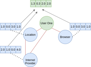
Graph convolutional networks are an extension of traditional convolutional neural networks that take advantage of the graph structure. As a quick recap, a graph structure is made of a collection of nodes, with edges connecting nodes that have a relationship together. For instance, if a node exists for a user on a website, that node could be connected to an IP address, location, and service provider as shown in the figure below.

Simple graph for a user on a website, the nodes are circles and the edges are red lines

Notice that internet provider and browser are not connected with an edge as they are not related, however location and internet provider are connected as they are related. The graph above shows all the nodes directly connected to the node "User One" with an edge; we'll call these nodes neighbours.

In graph convolutional networks, for each node $x_{i}$ in the graph, the neighbours attribute values are aggregated(using an average function in most instances) to give us a node representation. The aggregation implies that a node can be accurately represented by an aggregation function over its neighbours, however, there are no real studies focusing on discovering a very effective aggregate function. Nonetheless, the use of an aggregation function enables us to have a node representation of the same size, regardless of the number of neighbours, thus enabling us to feed the representation into a neural network. An average aggregation function for the node "User One" can be seen in the figure below(note: while not shown in the figure, the aggregation also includes the node's own attribute vector).

An average aggregation function on the neighbors of node "User One".

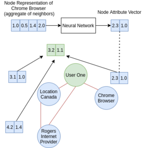
This process is repeated for every node in the graph, and thus we will have a node representation for each node. For each node, the node representation is fed into a single or a multi-layer neural network. The output of the neural network could be a vector representation or a classification label that can be learned in a supervised manner. In a multi-layer GCN, the output of the neural network for each input node representation will become the node's attribute vector. The aggregation step is then repeated for the new node neighbours attribute vectors and fed into the next layer of the GCN. Notice that by increasing the number of GCN layers, we can increase the number of neighbours used for representing each node. Taking the figure above as an example, while in the first layer, only browser, location, and internet provider made up the representation of User One, in the second layer, User ones node representation is made of the aggregate of browsers, location, and internet providers neighbour aggregates(recall how the aggregation is done for each node in the graph). Thus we can dictate the degrees of neighbours used to classify some label by defining the number of GCN layers. The figure below aims to make this clearer.

An example for bridging the intuition behind multi-layer GCNs

The Pseudo-code for learning a graph convolutional networks can thus be defined as follows:

1. For each node in the graph, calculate its node representation by taking the aggregate of its neighbors attribute vectors
2. For each node in the graph, pass the node representation into a neural network to either:
   • a) Classify the node and back-propagate the loss to update the weights
   • b) Form a new attribute vector for the node
3. If b) was taken, re-do steps 1 and 2.

Relational Graph Convolutional Networks

The use of GCNs in relational graphs such as knowledge bases will not provide good results as there is no differentiation between different type of relations. That is, all neighbouring nodes are aggregated into one node representation without differentiating between edge type(relation). Since only one representation is used for each node, only one set of weights are used in the neural network. This can be seen in the GCN neural network propagation function below(bias term emitted for simplicity):

$$h_{i}^{l+1}=\sigma (\sum _{j\in N_{i}}{\frac {1}{c_{ij}}}h_{j}^{(l)}W^{(l)})$$

Where $h_{i}$ is the output of the layer $l$ for node $i$, $\sigma$ is the activation function of the layer, $N_{i}$ is the set of neighbouring nodes, ${\frac {1}{c_{ij}}}$ is a normalisation constant, and $W$ is the trainable weights of the layer.

The R-GCN paper fixes this issue by representing each node by multiple aggregation vectors, one for each edge type connected to the node. This can be seen in the figure below.

Aggregation based on the relation type in R-GCN, forming a node representation for User One for each relation type.

Given that we now have more than one node representation vector for each node, we need to feed each representation into a neural network. This is where the authors of R-GCN make another change to the GCN paper; instead of using one set of neural network weights for all node representations, each relation type will be given its own set of weights. This can be seen in R-GCN neural network propagation function below, where $R$ is the set of relations a node $i$ has with its neighbours:

$$h_{i}^{l+1}=\sigma (W_{0}^{(l)}h_{i}^{(l)}+\sum _{r\in R}\sum _{j\in N_{i}^{r}}{\frac {1}{c_{ir}}}h_{j}^{(l)}W_{r}^{(l)})$$

Another change to the GCN paper can be seen in the equation above, where $W_{0}^{(l)}h_{i}^{(l)}$ defines weights for the nodes own attribute vector. This is made to differentiate between the neighbouring nodes values, and the value of the node itself.

While the additions discussed in this section already allow the model to be used for entity prediction and link prediction for knowledge bases, this new formulation does have its own problems which the authors of R-GCN rectify. Namely, the higher the number of relations in a dataset, the higher the number of parameters in the model; this can lead to over fitting on rare relations and models of large size. This issue was addressed by the authors by using two methods, of which one will be discussed on this page(the other method is beyond my mathematical scope). This method is basis decomposition, which in essence is a weight sharing scheme. In basis decomposition, we define $B$ number of weights $V$ to use, and a coefficient $a$ for each relation $r$ and weight $V$, we then take the linear combination of the coefficients and weights to form our neural network weights $W$. This can be more clearly seen in the equation below.

$$W_{r}^{(l)}=\sum _{b=1}^{B}a_{rb}^{(l)}V_{b}^{(l)}$$

It can also be noted, that by increasing B, the number of parameters in the model will be increased, and by decreasing B, we decrease the number of parameters in the model, which will reduce the computational complexity of the model. With the establishment of the above concepts, Figure 3 in shows how the R-GCN can be used for entity classification and link prediction.

Conclusion

In summary, the authors of the GCN paper introduced a method of applying convolutions on graph structures. The authors of the R-GCN paper then devised a method built on the GCN framework, of using convolutions on relational graph structures such as knowledge graphs. The authors then used two regularisation methods to ensure that their R-GCN method does not over fit.

To Add

Put links and content here to be added. This does not need to be organized, and will not be graded as part of the page. If you find something that might be useful for a page, feel free to put it here.