Course:CPSC532:StaRAI2020:GraphNeuralNetworks

Graph Neural Networks

Graph neural networks (GNNs) are deep learning based methods that operate on graph domain.

Authors: Melika Farahani, Mohamad Amin Mohamadi

Abstract

Deep learning has revolutionized many machine learning tasks in recent years, ranging from image classification and video processing to speech recognition and natural language understanding. The data in these tasks are typically represented in the Euclidean space. However, there is an increasing number of applications where data are generated from non-Euclidean domains and are represented as graphs with complex relationships and interdependency between objects. The complexity of graph data has imposed significant challenges on existing machine learning algorithms. Recently, many studies on extending deep learning approaches for graph data have emerged. In this page, we provide a comprehensive overview of graph neural networks (GNNs) in data mining and machine learning fields. We propose a new taxonomy to divide the state-of-the-art graph neural networks into four categories, namely recurrent graph neural networks, convolutional graph neural networks, graph autoencoders, and spatial-temporal graph neural networks.

Content

Definition of GNN

Many underlying relationships among data in several areas of science and engineering, e.g., computer vision, molecular chemistry, molecular biology, pattern recognition, and data mining, can be represented in terms of graphs. The graph neural network (GNN) model extends existing neural network methods for processing the data represented in graph domains. The GNN model, which can directly process most of the practically useful types of graphs, e.g., acyclic, cyclic, directed, and undirected, implements a function $tau(G,n)\in IR$ m that maps a graph $G$ and one of its nodes $n$ into an $m$-dimensional Euclidean space. A supervised learning algorithm is derived to estimate the parameters of the proposed GNN model. The target of GNN is to learn a state embedding $h_{v}\in R^{s}$ which contains the information of neighbourhood for each node. The state embedding $h_{v}$ is an $s$-dimension vector of node $v$ and can be used to produce an output $o_{v}$ such as the node label.

GNN Groups and Categorization

Graph neural networks are categorized into four groups: recurrent graph neural networks, convolutional graph neural networks, graph autoencoders, and spatial-temporal graph neural networks.

• Recurrent graph neural networks (RecGNNs) mostly are pioneer works of graph neural networks. RecGNNs aim to learn node representations with recurrent neural architectures. They assume a node in a graph constantly exchanges information/message with its neighbors until a stable equilibrium is reached. RecGNNs are conceptually important and inspired later research on convolutional graph neural networks. In particular, the idea of message passing is inherited by spatialbased convolutional graph neural networks.
• Convolutional graph neural networks (ConvGNNs) generalize the operation of convolution from grid data to graph data. The main idea is to generate a node $v$’s representation by aggregating its own features $x_{v}$ and neighbors’ features $x_{u}$, where $u\in N(v)$. Different from RecGNNs, ConvGNNs stack multiple graph convolutional layers to extract high-level node representations. ConvGNNs play a central role in building up many other complex GNN models.
• Graph autoencoders (GAEs) are unsupervised learning frameworks which encode nodes/graphs into a latent vector space and reconstruct graph data from the encoded information. GAEs are used to learn network embeddings and graph generative distributions. For network embedding, GAEs learn latent node representations through reconstructing graph structural information such as the graph adjacency matrix. For graph generation, some methods generate nodes and edges of a graph step by step while other methods output a graph all at once.
• Spatial-temporal graph neural networks (STGNNs) aim to learn hidden patterns from spatial-temporal graphs, which become increasingly important in a variety of applications such as traffic speed forecasting, driver maneuver anticipation, and human action recognition. The key idea of STGNNs is to consider spatial dependency and temporal dependency at the same time. Many current approaches integrate graph convolutions to capture spatial dependency with RNNs or CNNs to model the temporal dependency.

Why are graph neural networks worth investigating?

• The standard neural networks like CNNs and RNNs cannot handle the graph input properly in that they stack the feature of nodes by a specific order. However, the output of GNNs is invariant for the input order of nodes.
• An edge in a graph represents the information of dependency between two nodes. In the standard neural networks, the dependency information is just regarded as the feature of nodes. However, GNNs can do propagation guided by the graph structure instead of using it as part of features.
• The standard neural networks have shown the ability to generate synthetic images and documents by learning the distribution of data while they still cannot learn the reasoning graph from large experimental data. However, GNNs explore to generate the graph from non-structural data like scene pictures and story documents, which can be a powerful neural model for further high-level AI.

GNN Outputs

With the graph structure and node content information as inputs, the outputs of GNNs can focus on different graph analytics tasks with one of the following mechanisms:

• Node-level outputs relate to node regression and node classification tasks. RecGNNs and ConvGNNs can extract high-level node representations by information propagation/graph convolution. With a multi-perceptron or a softmax layer as the output layer, GNNs are able to perform node-level tasks in an end-to-end manner.
• Edge-level outputs relate to the edge classification and link prediction tasks. With two nodes’ hidden representations from GNNs as inputs, a similarity function or a neural network can be utilized to predict the label/connection strength of an edge.
• Graph-level outputs relate to the graph classification task. To obtain a compact representation on the graph level, GNNs are often combined with pooling and readout operations.

Formalization

Graphs and Graph related data

A graph is represented as $G=(V,E)$ where $V$ is the set of vertices or nodes (we will use nodes throughout the paper), and $E$ is the set of edges. Let $v_{i}\in V$ to denote a node and $e_{ij}=(v_{i},v_{j})\in E$ to denote an edge pointing from $v_{j}$ to $v_{i}$. The neighborhood of a node v is defined as $N(v)=\{u\in V|(v,u)\in E\}$. The adjacency matrix $A$ is a $n\times n$ matrix with $A_{ij}=1$ if $e{ij}\in E$ and $A_{ij}=0$otherwise. A graph may have node attributes $X$, where $X\in R^{n\times d}$ is a node feature matrix with $x_{v}\in R^{d}$ representing the feature vector of a node $v$. Meanwhile, a graph may have edge attributes $X_{e}$, where $X_{e}\in R^{m\times c}$ is an edge feature matrix with $x_{v,u}^{e}\in R^{c}$ representing the feature vector of an edge $(v,u)$.

Graph neural networks

Let $H,O,X,X_{N}$be the vectors constructed by stacking all the states, all the outputs, all the features, and all the node features, respectively. Then we have a compact form as: $H=F(X,H)$, $O=G(H,X_{N})$. Now that $H$is a fixed point, we can iteratively use the equation $H^{t+1}=F(H^{t},X)$ to retrieve it. This value is uniquely defined under the assumption of F being a contraction map.

Learning a GNN

When we have the framework of GNN, the next question is how to learn the parameters of $f$ and $g$. With the target information ($t_{v}$ for a specific node) for the supervision, the loss can be written as follow:

$loss=\sum _{i=1}^{p}(t_{i}-o_{i})$

where $p$ is the number of supervised nodes. The learning algorithm is based on a gradient-descent strategy and is composed of the following steps:

• The states $h_{v}^{t}$ are iteratively updated by until a time $T$. They approach the fixed point solution of $H(T)\approx H$H(T) ≈ H.
• The gradient of weights $W$ is computed from the loss.
• The weights $W$ are updated according to the gradient computed in the last step.

Training frameworks and limitations

Limitations of the basic GNN

Though experimental results showed that GNN is a powerful architecture for modeling structural data, there are still several limitations of the original GNN.

1. Firstly, it is inefficient to update the hidden states of nodes iteratively for the fixed point. If relaxing the assumption of the fixed point, we can design a multi-layer GNN to get a stable representation of node and its neighborhood.
2. Secondly, GNN uses the same parameters in the iteration while most popular neural networks use different parameters in different layers, which serve as a hierarchical feature extraction method. Moreover, the update of node hidden states is a sequential process which can benefit from the RNN kernel like GRU and LSTM.
3. Thirdly, there are also some informative features on the edges which cannot be effectively modeled in the original GNN. For example, the edges in the knowledge graph have the type of relations and the message propagation through different edges should be different according to their types.
4. Lastly, it is unsuitable to use the fixed points if we focus on the representation of nodes instead of graphs because the distribution of representation in the fixed point will be much smooth in value and less informative for distinguishing each node.

Therefore, different variants of the basic GNN model have been developed to address these problems, some of which we have mentioned in the GNN categorization section.

GNN Training Framework

Many GNNs (e.g., ConvGNNs) can be trained in a (semi-) supervised or purely unsupervised way within an end-to-end learning framework, depending on the learning tasks and label information available at hand.

• Semi-supervised learning for node-level classification. Given a single network with partial nodes being labeled and others remaining unlabeled, ConvGNNs can learn a robust model that effectively identifies the class labels for the unlabeled nodes.
• Supervised learning for graph-level classification. Graph-level classification aims to predict the class label(s) for an entire graph. The end-to-end learning for this task can be realized with a combination of graph convolutional layers, graph pooling layers, and/or readout layers. While graph convolutional layers are responsible for exacting high-level node representations, graph pooling layers play the role of downsampling, which coarsens each graph into a sub-structure each time. A readout layer collapses node representations of each graph into a graph representation. By applying a multi-layer perceptron and a softmax layer to graph representations, we can build an end-to-end framework for graph classification.
• Unsupervised learning for graph embedding. When no class labels are available in graphs, we can learn the graph embedding in a purely unsupervised way in an end-to-end framework. These algorithms exploit edge-level information in two ways. One simple way is to adopt an autoencoder framework where the encoder employs graph convolutional layers to embed the graph into the latent representation upon which a decoder is used to reconstruct the graph structure.

GNN Samples

GNN Applications Examples

1. Recommender Systems: A standard use case is to model interactions within the graph of users and items, learn node embeddings with some form of negative sampling loss, and use KNN index to retrieve similar items to the given users in real-time.
   

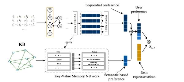
   Baocheng Wang et al used this model for Sequential Recommendation. This consists of a key-value memory network (KV-MN) and a graph neural network (GNN). By linking existing external knowledge base entities with items in recommender systems, key-value memory networks are able to incorporate KB knowledge, and the GNN component is used to capture complex transitions. By combining a GNN and KV-MN, the final user preference is a combination of current and global interests.
2. Computer Vision: Understanding a visual scene goes beyond recognizing individual objects in isolation. Relationships between objects also constitute rich semantic information about the scene. The images that contain these objects can also benefit from GNNs. In a recent work from Danfei XU et al, they explicitly model the objects and their relationships using scene graphs, a visually-grounded graphical structure of an image.
   

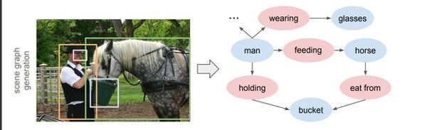
   They propose a scene graph generation model that takes an image as input, and generates a visually-grounded scene graph (second row, right) that captures the objects in the image (blue nodes) and their pairwise relationships (red nodes).

Annotated Bibliography

• [1] The graph neural network model (Franco Scarselli et al)
• [2] A Comprehensive Survey on Graph Neural Networks (Zonghan Wu)
• [3] Graph Neural Networks: A Review of Methods and Applications (Jie Zhou et al)
• [4] Top Applications of Graph Neural Networks 2021 (Sergei Ivanov)
• [5] Knowledge-Enhanced Graph Neural Networks for Sequential Recommendation (Baocheng Wang et al)
• [6] Scene Graph Generation by Iterative Message Passing (Danfei Xu et al)

To Add

Put links and content here to be added. This does not need to be organized, and will not be graded as part of the page. If you find something that might be useful for a page, feel free to put it here.