Course:CPSC522/Long Short Term Memory Networks

Long Short-Term Memory Networks (LSTMs)

LSTM is a type of Recurrent Neural Network (RNN) that is designed to process sequential data by selectively retaining or forgetting information from previous time steps, making it particularly useful for tasks such as speech recognition, natural language processing (NLP), and time series prediction.

Principal Author: Harshinee Sriram

Collaborators:

Abstract

This article provides an overview of LSTMs, starting from an introduction, a description of an LSTM unit and its gates, followed by how the LSTM network works. Next, it describes the different variants of LSTMs, and ultimately concludes by discussing the various applications of LSTMs.

Builds on

• Recurrent Neural Networks (RNNs) are a type of neural network designed to process sequential data by retaining and using information from previous inputs.
• Artificial neural networks (ANNs) are computing systems that are designed to simulate the behavior of the human brain, capable of learning from data and making predictions or decisions.

Related Pages

• Gated Recurrent Units (GRUs) are a type of ANN that are similar to LSTMs, but have a simpler structure by combining the reset and update gates.
• Natural Language Processing (NLP) is a field of computer science and artificial intelligence that deals with the interaction between computers and humans using natural language.
• Transformer models are a type of neural network architecture that uses self-attention mechanisms to process sequential data in parallel, unlike LSTMs which process data sequentially using memory cells.

Content

Introduction to LSTMs and the motivation behind developing them

RNNs are a type of neural networks designed to handle sequential data, where the output depends on the previous inputs. Although RNNs have shown success in various text-based and speech-based applications, they suffer from the problem of vanishing gradients, where the gradients become too small to update the weights of the network, leading to poor performance. LSTMs were introduced in the work by Hochreiter and Schmidhuber (1997) as an extension of the standard RNN architecture to overcome this vanishing gradient problem by allowing the network to decide what information to keep and what to discard. This selective memory retention helps LSTMs handle long-term dependencies in sequential data better than RNNs as they can forget instances in the input sequence that are of lesser significance. As a result, LSTMs have achieved better performance than RNNs in tasks such as speech recognition, NLP, and music generation.

Figure 1a: The anatomy of an LSTM unit. Source: https://www.analyticsvidhya.com/blog/2022/03/an-overview-on-long-short-term-memory-lstm/#:~:text=Structure%20Of%20LSTM&text=A%20conventional%20LSTM%20unit%20consists,values%20over%20arbitrary%20time%20intervals.

Understanding LSTMs

Figure 1b: A deeper dive into the LSTM unit anatomy. Source: https://medium.com/@antonio.lopardo/the-basics-of-language-modeling-1c8832f21079

Notations

Following are the notations that will be used in this article. These notations will be further explained in the next sub-sections.

• The current timestep (processing during a certain moment) is denoted with $t$, whereas the previous timestep is referred to as $t-1$.
• A hidden state $h$, where the current hidden state is $h_{t}$ whereas the previous hidden state is $h_{t-1}$.
• An input vector $x$, where the current input vector is $x_{t}$.
• A final cell state $C$ (also known as the context vector) that stores the long-term memory. $C_{t-1}$ refers to the long-term memory in the previous timestep whereas $C_{t}$ refers to the current long-term memory.
• A temporary scaled version of the new long-term state $C'$ that is used to compute the final cell state $C$. Similar to the notation above, this temporary cell state at the current timestep is denoted as $C_{t}'$.
• A weight vector $W$ and a bias vector $b$.
• A forget gate at the current timestep $f_{t}$ that contains the weight vector $W_{f}$ and the bias vector $b_{f}$.
• An input gate at the current timestep $i_{t}$ that contains the weight vector $W_{i}$ and the bias vector $b_{i}$.
• An output gate at the current timestep $o_{t}$ that contains the weight vector $W_{o}$ and the bias vector $b_{o}$.
• The sigmoid ($\sigma$) and tanh (tanh) activation functions.
• Pointwise multiplication is denoted with $\cdot$
• Matrix multiplication is denoted with $\times$
• The Hadamard multiplication (a type of element-wise multiplication applied to two matrices or vectors of the same dimension) is denoted with $*$.

The anatomy of an LSTM unit

Figure 1a shows the anatomy of an LSTM unit whereas Figure 1b explicitly mentions how the internal logic of this unit works. At a high level, an LSTM unit consists of three gates (forget, input, and output) and a memory cell. The three gates have been further described as follows:

1. The forget gate controls how much old information is discarded from the previous cell state $(C_{t-1})$ using a sigmoid function. For each component in $C_{t-1}$, the forget gate looks at the concerning hidden state $h_{t-1}$ and the input state $x_{t}$ to produce a number in the $[0,1]$ range. The concerning equations are as follows:
   1. Determining what inputs are discarded: $f_{t}=\sigma (W_{f}\,\times \,[h_{t-1},x_{t}]+b_{f})$
2. The input gate decides which of the input values should alter the current memory $(C_{t})$. It consists of a sigmoid function $(\sigma )$ and a tanh function. The sigmoid function outputs a value between 0 and 1 to indicate how much of the input should be selected whereas the tanh function takes the selected input and decides how much of it should be added to the cell state. Note that the inputs to both $C_{t}$ and $i_{t}$ are the same as those sent to $f_{t}$. The resulting equations are as follows:
   1. Deciding the input values to select at timestep $t$: $i_{t}=\sigma (W_{i}\,\times \,[h_{t-1},x_{t}]+b_{i})$
   2. Deciding what information the new cell state should contain at timestep $t$: $C_{t}'=tanh(W_{c}\,\times \,[h_{t-1},x_{t}]+b_{c})$
   3. Computing the current cell state $C_{t}=f_{t}\,\cdot \,(C_{t-1})+i_{t}\,\cdot \,C_{t}'$
3. The output gate controls how much information is outputted from the memory cell. Similar to the input gate, it contains a sigmoid function and a tanh function and they have the same purpose i.e. the sigmoid function determines how much of the input should be selected whereas the tanh function scales the cell state that is about to be passed on to the next LSTM unit or to the output layer. The following shows the equations involved in this step:
   1. Deciding the input values to select at timestep $t$: $o_{t}=\sigma (W_{o}\,\times \,[h_{t-1},x_{t}]+b_{o})$
   2. Finalizing the next hidden state at timestep $t$: $h_{t}=o_{t}\,*\,tanh(C_{t})$

How do these LSTM units work?

The inner working of an LSTM unit has three main steps, which are explained below:

1. Generating the forget gate $(f_{t})$ output: First, we decide what bits in the current cell state $(C_{t})$ need to be removed (or kept) given both the previous hidden state $(h_{t-1})$ and the new input data $(x_{t})$. Both $h_{t-1}$ and $x_{t}$ are sent to a neural network within the forget gate $(W_{f}\,\cdot \,[h_{t-1},x_{t}]+b_{f})$ that generates a vector where each element lies in the $[0,1]$ interval (made certain by the sigmoid $(\sigma )$ activation). This network is trained so that an output close to 0 refers to an irrelevant input component whereas an output close to 1 refers to a relevant component. These output values are then pointwise multiplied with the previous cell state i.e. $f_{t}\,\cdot \,(C_{t-1})$. This means that the input components in the previous cell state that are now deemed irrelevant by the forget gate network are multiplied by a number close to 0 (to reduce their influence in the future) while those deemed relevant are multiplied by a number close to 1.
2. Generating the current cell state $(C_{t})$ and input gate $(i_{t})$ outputs: Next, we determine what new information needs to be added to the current cell $(C_{t})$ state given the previous hidden state $(h_{t-1})$ and new input data $(x_{t})$. The output vector from this tanh activated neural network $(C_{t}')$ contains information from the new input data given the context from the previous hidden state. However, there is no actual assessment of the new input data to check if it is even worth remembering. This is why the input gate $(i_{t})$ is used, as it identifies the components in $x_{t}$ that are worth remembering. It follows the same mechanism as $f_{t}$ as it outputs values in the $[0,1]$ interval due to the sigmoid activation. Next, $C_{t}'$ and $i_{t}$ are multiplied and added to the previously computed $f_{t}\,\cdot \,(C_{t-1})$ to form the current cell state $C_{t}$, which updates the long-term memory of the network.
3. Generating the output gate $(o_{t})$ and next hidden state $(h_{t})$ outputs: We cannot just output the $C_{t}$ we received after the previous step because it contains all information kept since the beginning. This is similar to asking someone a specific question on Transformers and they begin their response by talking about probabilities. To prevent this from happening, the output gate $(o_{t})$ is used to act as a filter. This takes the same inputs as those in $f_{t}$ and processes them in a similar manner, resulting in a sigmoid activation influenced output that lies in the $[0,1]$ interval. Next, $C_{t}$is passed through a tanh function to force the values into the $[-1,1]$ interval. The $o_{t}$ gate is then applied to this $C_{t}$ with a Hadamard multiplication of the two to ensure that only necessary information is sent as output, resulting in the next hidden state $(h_{t})$.

Note: The steps above are repeated many times, depending on the sequence length. For instance, if you are trying to predict the price of a house given its price from the last 20 years, this process will be repeated 20 times. But, the output of the LSTM unit is still a hidden state $(h_{t})$, which isn't the final output. To convert it to a final output, a linear layer needs to be added.

Variants of LSTMs

Over the years, several variants of LSTMs have been introduced to address specific problems and improve performance. Here are some of the most common variants:

• Bidirectional-LSTM (BiLSTM) networks: A traditional LSTM network processes input sequences unidirectionally where the input for the next LSTM unit is determined by the output of the previous LSTM unit (see Figure 2). The main disadvantage of unidirectional LSTMs is that they can only capture information from the past or the future, but not both. This means that they may miss important context that is only available in the opposite direction. For example, when processing a sentence, the meaning of a word can be influenced by the words that come before and after it. Bidirectional LSTMs were developed by Schuster et. al. (1997) to address this limitation by processing the input sequence in both directions, using two separate LSTMs that run in opposite directions (see Figure 3). This allows the model to capture both past and future contexts and better understand the meaning of each word in the sentence. By combining the outputs of the two LSTMs, a bidirectional LSTM can produce a more accurate representation of the input sequence. This is particularly useful in NLP applications where the meaning of a word can depend on the context in which it appears.

Figure 2: Unidirectional LSTMs Source: https://medium.com/@raghavaggarwal0089/bi-lstm-bc3d68da8bd0

Figure 3: Bidirectional LSTMs (BiLSTMs)
Source: https://medium.com/@raghavaggarwal0089/bi-lstm-bc3d68da8bd0

• Convolutional LSTM (ConvLSTM) networks: Unlike a traditional LSTM that treats the input as a flat vector, ConvLSTMs process inputs with spatial structures (such as images or videos) using the convolutional operation on the input sequence (see Figure 4). The key difference between a traditional LSTM network and a ConvLSTM network is the addition of convolutional layers to the input, forget, and output gates. In a traditional LSTM, these gates are usually implemented as fully connected layers, which can be slow and memory-intensive for large inputs. By adding convolutional layers to these gates, ConvLSTMs operate on input data with less computation and memory requirements. Another important feature of ConvLSTM is its ability to learn spatio-temporal patterns. By incorporating convolutional layers, the model can capture both spatial and temporal dependencies in the input data. This makes ConvLSTMs particularly effective for tasks such as video classification, where the goal is to recognize patterns in both time and space. To learn more about ConvLSTMs, refer to the work by Shi et al. (2015) that introduced them.

Figure 4: The anatomy of a ConvLSTM unit.
Source: Shi, Changjiang, Zhijie Zhang, Wanchang Zhang, Chuanrong Zhang, and Qiang Xu. "Learning multiscale temporal–spatial–spectral features via a multipath convolutional LSTM neural network for change detection with hyperspectral images." IEEE Transactions on Geoscience and Remote Sensing 60 (2022): 1-16.

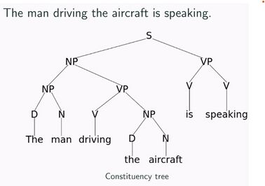
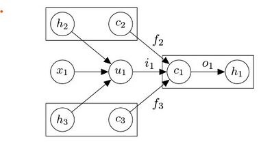
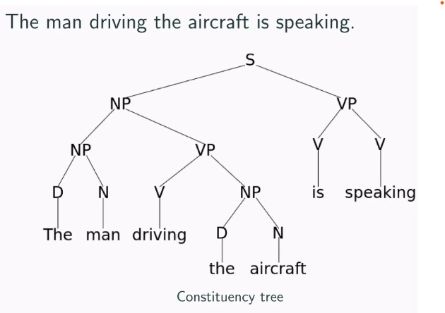
• Tree LSTM (TLSTM) networks: TLSTM networks are a variant of LSTM networks that are used for processing tree-structured data, such as natural language syntax trees (see Figure 5). The main difference between a TLSTM and a traditional LSTM lies in the way input information is processed and propagated through the network. In a traditional LSTM, input information is processed sequentially and propagated along a linear chain of LSTM cells. In contrast, a TLSTM operates on a tree structure, where each node represents a word or phrase in the sentence, and the edges represent the syntactic dependencies between these nodes. At each node, a TLSTM computes a cell state that takes into account the information from the current node and its child nodes (see Figure 6). This allows a TLSTM to capture the hierarchical structure of language and to better model long-range dependencies. TLSTMs have the following two key aspects to their design:
  • TLSTMs use a modified gating mechanism called the "composition gate" to combine information from child nodes. This gate allows a TLSTM to selectively incorporate information from child nodes based on their relevance to the current node, which helps prevent the propagation of irrelevant information.
  • TLSTMs also use a "recursive cell" that computes the cell state for each node based on the cell states of its child nodes. This recursive cell allows a TLSTM to propagate information from the leaves of the tree up to the root, enabling it to model dependencies over longer distances.
    

    Figure 5: An example for a Natural Language syntax tree.
    Source: https://www.slideshare.net/tuvistavie/tree-lstm
    

    Figure 6: Composing the memory cell $c_{1}$ and hidden state $h_{1}$of a Tree-LSTM unit with two children (subscripts 2 and 3). Labeled edges correspond to gating by the indicated gating vector, with dependencies omitted for compactness.
    Source: Tai, Kai Sheng, Richard Socher, and Christopher D. Manning. "Improved semantic representations from tree-structured long short-term memory networks." arXiv preprint arXiv:1503.00075 (2015).

One limitation of TLSTMs is that they can be computationally expensive due to the need to recursively compute the cell state at each node. To address this issue, various approximations and optimizations have been proposed, such as using a fixed-depth tree traversal or incorporating convolutional operations. There are two tree-based extensions to the traditional unidirectional LSTM architecture:

• Child-sum Tree LSTMs: Child-sum Tree LSTMs work by recursively computing hidden states for each node in the tree. At each level of the tree, the hidden state of each node is computed by combining the hidden states of its child nodes in an unordered manner. This is done using a child-sum operation, where the hidden state of a node is the sum of the hidden states of its child nodes and all child nodes share the same set of parameters.
• N-ary Tree LSTMs: Compared to child-sum tree LSTMs, N-ary Tree LSTMs discriminate among child node positions using a weighted sum of their hidden nodes, implying an ordering of these child nodes. Additionally, different child nodes contain different sets of parameters. Hence, to compute the output of a particular node, N-ary Tree LSTMs use an additional gating mechanism known as the "node-gate" which helps the model determine which children nodes are most relevant to the computation of the parent node. This node-gate is responsible for computing a weight for each child node's hidden state, which are then used to calculate a weighted sum of the child hidden states that are fed to the LSTM cell.

To learn more, kindly refer to the work by Tai et al. (2015).

Figure 7: A peephole LSTM unit
Source: https://medium.com/nerd-for-tech/what-is-lstm-peephole-lstm-and-gru-77470d84954b

Figure 8: A GRU unit
Source: https://medium.com/nerd-for-tech/what-is-lstm-peephole-lstm-and-gru-77470d84954b

• Peephole LSTM networks: In traditional LSTMs, the gates (input, forget, and output) take the current input ($x_{t}$) and the previous hidden state ($h_{t-1}$), but not directly from the previous cell state/context vector ($C_{t-1}$). On the other hand, peephole LSTM networks add a set of peephole connections to the cell state $C$, allowing the gates to take in information about the previous cell state directly (see Figure 7). By allowing the gates to have direct access to the cell state, peephole LSTM networks can more accurately decide what information to keep and what information to discard. This additional information from the previous cell state allows the model to better capture long-term dependencies and helps prevent the vanishing gradient problem that can still occur to some extent in traditional LSTMs. To learn more, kindly refer to the work by Gers et al. (2000).

• Gated Recurrent Unit (GRU) Networks: GRU networks are a simpler variant of LSTM networks. In contrast to LSTMs, GRUs have two gates: an update gate (that combines the input and forget gates) and a reset gate. The update gate determines how much of the previous hidden state should be retained whereas the reset gate decides how much of the new input should be forgotten. The output of the reset gate is combined with the current input and fed to a hyperbolic tangent function that produces the candidate activation. This candidate activation is then combined with the output of the update gate to generate the new hidden state. Figure 8 shows the internal structure of a GRU unit and Figure 9 shows how this unit operates. To learn more, kindly refer to this article.

One key advantage of GRUs is that they have fewer parameters than LSTMs, which makes them easier to train and become more computationally efficient. Additionally, since GRUs have fewer gates than LSTMs, they can be less prone to overfitting and more robust to noise in the input data. However, this simplicity can also be a disadvantage in certain scenarios, as GRUs may not be able to capture as much long-term dependencies as LSTMs.

Figure 9: A GIF showing how a GRU unit operates. Source: https://medium.com/nerd-for-tech/what-is-lstm-peephole-lstm-and-gru-77470d84954b

Application of LSTMs

Natural language processing (NLP)

Figure 10: An example of long translation produced by the LSTM alongside the ground truth translations. Source: Sutskever, Ilya, Oriol Vinyals, and Quoc V. Le. "Sequence to sequence learning with neural networks." Advances in neural information processing systems 27 (2014). This reference is used twice on this page.

One of the primary applications of LSTMs in NLP is language modeling, which involves predicting the the next word in a sequence given the previous words. Under this general application, LSTMs have been used for speech recognition, where they are trained on acoustic features to predict the corresponding phonemes or words. For example, the work by Graves et al. (2013) showed that LSTMs outperformed traditional HMM-based methods in both phoneme recognition and word recognition tasks. Another application is machine translation, where they have been used to model the sequence-to-sequence mapping between two languages (Bahdanau et al., 2014; Sutskever et al., 2014). Figure 10 from Sutskever et al., 2014 shows how the resulting sentence from the LSTM networks compares against the ground truth. Lastly, LSTMs have also been used for text classification tasks, such as sentiment analysis (Wang et al., 2016), topic modeling (Tang et al., 2015), and named entity recognition, where they are trained to predict the type of entity (e.g. person, organization, location) mentioned in a text (Lample et al., 2016).

Time series prediction

LSTM networks have been used for time series prediction in the field of finance, where they have predicted stock prices and financial markets (Moghar and Mhamed, 2020; Bukhari et al., 2020; Roondiwala et al., 2017). LSTMs have also been applied in weather forecasting (Tao et al., 2021; Chang et al., 2020), traffic prediction (Kang et al., 2017; Liu et al., 2017), and energy demand forecasting (Le et al., 2019).

Figure 11: How a Vision Deep CNN + Language Generating RNN (LSTM) network extracts relevant features from an image for caption generation. Source: Vinyals, Oriol, Alexander Toshev, Samy Bengio, and Dumitru Erhan. "Show and tell: A neural image caption generator." In Proceedings of the IEEE conference on computer vision and pattern recognition, pp. 3156-3164. 2015.

Image and video captioning

One of the earliest use of LSTMs in image captioning was introduced in the work by Vinyals et al. (2015). This paper proposed an end-to-end neural network model that learns to generate captions for images. The model used a convolutional neural network (CNN) to extract features from the input image, which were then fed to an LSTM network that generated a corresponding caption (see Figure 11). This approach achieved state-of-the-art results on standard image captioning benchmarks. Similarly, in video captioning tasks, LSTMs have been used along with CNNs to extract relevant spatio-temporal features (Donahue et al., 2015). Another interesting application of LSTMs in image and video captioning is the use of attention mechanisms, which allow the model to focus on specific regions of the input image or video that are most relevant to generating the caption. One such model was developed by Xu et al. (2015), where attention was incorporated the LSTM-based image captioning model to improve the quality of generated captions.

Note: To learn more about how attention works in an LSTM network and if attention weights are a way to gauge input feature importance, refer to this article.

To Add

Put links and content here to be added. This does not need to be organized, and will not be graded as part of the page. If you find something that might be useful for a page, feel free to put it here.