Course:CPSC522/Generative Adversarial Networks

Generative Adversarial Networks

Generative Adversarial Networks (GAN) is a framework for training generative models that use deep neural networks. The approach simultaneously trains a generative model alongside an adversarial discriminative model. The discriminative model tries to determine whether a sample comes from the true data distribution or from the generative model, while the goal of the generative model is to fool the discriminative model.

Laplacian Generative Adversarial Networks (LAPGAN) combines the GAN method with the a specific representation of images called the Laplacian Pyramid. LAPGAN uses a sequence of convolutional networks to generate images incrementally, analogous to iteratively creating the Laplacian Pyramid representation.

Principal Author: Tian Qi (Ricky) Chen

Abstract

The aim of this wiki page is to introduce an approach to creating generative models (explained below) from a dataset. The created generative model should be able to generate samples from the same distribution as the provided dataset (the target distribution). This generative model can then be used to generate additional simulated data, which is extremely useful for applications that require (but lack) large amounts of data. This wiki page describes the recently proposed approach of Generative Adversarial Networks, a new method that is competitive with other existing methods when only a finite amount of samples from the target distribution are known. The approach is then built upon by the computer vision community to generate images, using a domain-specific image representation scheme, the Laplacian pyramid. This is then shown to have better generative performance using human evaluation testing.

Background

Knowledge about neural network architectures and probability distributions are assumed.

Generative vs Discriminative Models

We describe the differences between discriminative and generative models. Suppose we have some data $X$ and some signal $Y$, with joint distribution $p_{data}$. A discriminative model is a mapping from a value of $X$ to a signal $Y$. It does not care about the distribution $p_{data}$, only that there exist some boundaries separating the $X$'s that map to a certain value of $Y$ and the $X$'s that map to a different value of $Y$. On the other hand, a generative model tries to directly learn the distribution $p_{data}$. In doing so, it does not explicitly learn boundaries separating different signals, but instead learns the entire distribution, which can be used to infer about the signals $Y$.

The main advantage of a generative model over discriminative models is the ability to generate samples from the distribution $p_{data}$ (supposing that the generative model is able to perfectly model the distribution). So while discriminative models are simpler to train, and typically performs better on most supervised tasks, generative models are more expressive as it approximates the true data distribution.

Below, we discuss a framework that uses neural networks to construct a generative model. Neural networks have been shown to perform spectacularly as discriminative models, usually in a classification setting where the inputs are high dimensional. GAN is a method that takes advantage of the performance of neural networks as discriminative models to aid in the training of a generative neural network.

Generative Adversarial Networks

Generative Adversarial Networks (GAN) is a method for constructing a generative model that tries to learn the true distribution of the data, $p_{data}$. Let $G(z;\theta _{g})$ denote the generative model. In this case, $G$ is restricted to be a neural network with parameters $\theta _{g}$ that takes as input some noise $z$ with distribution $p_{z}$ and outputs a sample according to $G$'s distribution, $p_{g}$. Define a second (discriminative) neural network $D(x;\theta _{d})$ that outputs a single scalar representing the probability that $x$ came from the data rather than $p_{g}$.

The GAN approach simultaneously trains both $G$ and $D$. The discriminative model $D$ is trained to maximize the probability of assigning the correct label. Thus the probability output of $D$ should be high when the sample comes from $p_{data}$ and low when the sample comes from $p_{g}$. The proposed objective function for training $D$ is

$\max _{D}\mathbb {E} _{x\sim p_{data}}[logD(x)]+\mathbb {E} _{x'\sim p_{g}(x')}[log(1-D(x'))]$

However, since $p_{g}$ is only implicitly defined by the samples of the neural network $G$, there is no explicit formula. Instead, since $G$'s randomness comes from the prior $z$, the second term in the objective function can be reformulated in terms of $p_{z}$.

Additionally, the generative model $G$ is trained to fool the discriminative model into believing samples from $p_{g}$ are actually from $p_{data}$, thus $G$'s goal is to minimize the second term. This leads to the following minimax function:

$\min _{G}\max _{D}V(D,G)=\mathbb {E} _{x\sim p_{data}}[logD(x)]+\mathbb {E} _{z\sim p_{z}(z)}[log(1-D(G(z)))]$

The composition $D(G(z))$ is valid due to modularity of neural networks and that samples from $p_{data}$ and $p_{g}$ span the same space.

The training procedure alternates between updating $D$ whose distribution is visualized by the blue dashed line, and $G$ which maps the space of $z$ (lower horizontal line) to the space of $x$ (upper horizontal line); the distributions $p_{data}$ and $p_{g}$ are visualized by the dotted black line and solid green line, respectively.

Starting at (a), the generative model $G$ is near convergence and $D$ is a partially accurate classifier.

In (b), the discriminative model $D$ is updated, tending towards the optimizer $D^{*}(x)={\frac {p_{data}(x)}{p_{data}(x)+p_{g}(x)}}$. (This property is proven in the paper .)

(c) Once $D$ has been updated, the gradient for $G$ changes to flow to regions where $D$ classifies as data.

(d) After convergence, the optimal result is to have $p_{g}$ perfectly mimic the data distribution and $D$ to be unable to differentiate between the two distribution, ie. $D(x)=1/2$.

The only requirement for sampling from $G$ is the knowledge of a way to sample from $p_{z}$. Conversely, if iid samples of $z$ can be created, then the samples from $G$ are also iid. This property is an advantage of the GAN approach compared with other generative techniques that use MCMC-based sampling, where the samples are not independent.

Some sampling results

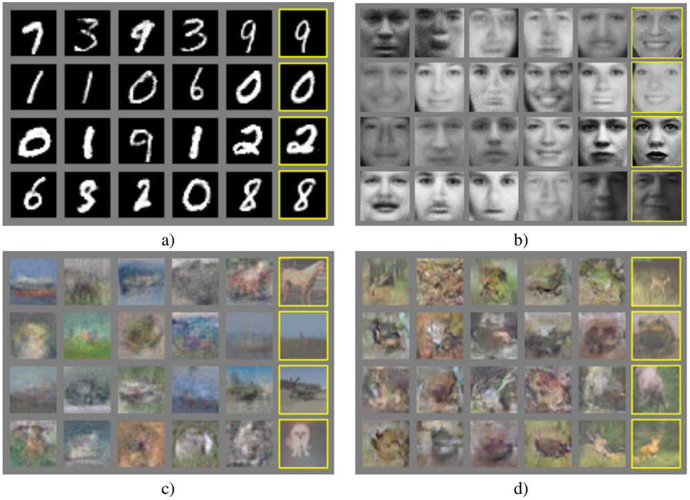
Below are some visualized samples from generative models trained using the GAN approach. The rightmost column shows the nearest neighbour training example of the sample displayed in the second rightmost column, to demonstrate that the model did not simply memorize the training set.

(a) MNIST is a dataset of handwritten digits in black and white. The generated samples are pretty good.

(b) TFD is a dataset of black and white faces. The generated samples definitely capture the structure of the human face, but some samples can still be identified as artificial. We see that some samples have very blurry shadows.

(c) CIFAR-10 is a dataset of 10 different classes of animals and automobiles. The generated samples look very blurred and certainly cannot fool the human eye.

(d) CIFAR-10 but with a different neural network model. This model uses convolutional layers whereas the networks for (a), (b), and (c) only use multilayer perceptrons. The results are still quite blurred and not recognizable as actual photos.

Overall, the GAN approach works for simple scenarios such as MNIST, but this is not particularly interesting. The approach fails as the complexity of the image increases, such as having added colour or varying objects. The resulting samples look blurred.

Laplacian Generative Adversarial Networks

Laplacian Pyramid

Illustration of the process of extracting the Laplacian pyramid of an image. The orange arrows are downsampling operators and the green arrows are upsampling operators. The original image is depicted on the left. The resulting $h_{k}$'s are the Laplacian pyramid.

Illustration of the process of reconstructing the image from a Laplacian pyramid. The green arrows are upsampling operators. By iteratively upsampling and appending the set of $h_{k}$'s, the original image is recovered on the left.

The Laplacian pyramid representation stores an image as a sequence of downsampled images, plus residuals for each downsampled image. This technique is typically used in image compression.

Let $d(\cdot )$ be a downsampling operator that takes a $j\times j$ image as input and produces a blurred image of half the size $j/2\times j/2$.

Let $u(\cdot )$ be an upsampling operator that takes a $j\times j$ image as input and produces a smoothed image of double the size $2j\times 2j$.

For an image $I$, first build a pyramid ${\mathcal {G}}(I)=[I_{0},I_{1},\dots ,I_{K}]$, where $I_{0}=I$ and $I_{k}$ is constructed by applying $k$ repeated applications of $d(\cdot )$. $K$ is the number of levels in the pyramid, chosen so that the final level is spatially small ($\leq 8\times 8$ pixels).

Then calculate coefficients $h_{k}$ for each level of the Laplacian pyramid by taking the different between the image at that level and the upsampled image at the lower adjacent level.

$h_{k}={\mathcal {L}}_{j}(I)={\mathcal {G}}_{k}(I)-u(G_{k+1}(I))=I_{k}-u(I_{k+1})$

The coefficient for the final level is simply the image itself ($h_{K}=I_{K}$).

Thus the Laplacian pyramid of image $I$ is defined by $d(\cdot ),u(\cdot ),\{h_{k}\}_{k=1}^{K}$. Reconstruction of the original image $I$ from the Laplacian pyramid coefficients uses the backward recurrence:

$I_{k}=u(I_{k+1})+h_{k}$

With $I_{0}=I$ being the original image. In order words, from the lowest level, the upsampling operator is applied repeated and the difference/residual is added to reconstruct the higher level.

The LAPGAN Approach

Laplacian Generative Adversarial Networks (LAPGAN) does not modify the GAN approach, but instead uses it at each level of a Laplacian pyramid. The LAPGAN approach is restricted to images. Instead of generating an image directly from scratch, the LAPGAN approach generates an image incrementally by generating the Laplacian pyramid.

One generative model is constructed for each level in the Laplacian pyramid, resulting in a set of convolutional network models $\{G_{0},\dots ,G_{K}\}$. The generative models at each level is responsible for capturing the distribution of the Laplacian coefficients $h_{k}$ when given an upsampled image of the lower adjacent level and a noise vector $z_{k}$. This yields the following model:

${\tilde {I}}_{k}=u({\tilde {I}}_{k+1})+{\tilde {h}}_{k}=u({\tilde {I}}_{k+1})+G_{k}(z_{k},u({\tilde {I}}_{k+1}))$

With ${\tilde {I}}_{K+1}=0$. With this formulation, all generative models except the final $G_{K}$ are conditional generative models that take the upsampled version of ${\tilde {I}}_{k+1}$ as the conditioning variable. As will be explained in later sections, the LAPGAN approach has the advantage of breaking the generation of an image into successive refinements, while also yielding a training method that trains each level of the pyramid independently.

Sampling

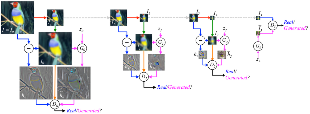
The sampling procedure of a $64\times 64$ image using the LAPGAN model is shown below.

Starting from a noise sample $z_{3}$ as input, $G_{3}$ generates ${\tilde {I}}_{3}$. This image is then upsampled (denoted by the green arrow) and, along with some noise vector $z_{2}$, fed as input to $G_{2}$ to produce ${\tilde {h}}_{2}$, which is then added to $I_{2}$ to produce ${\tilde {I}}_{2}$. This process is then repeated twice to produce ${\tilde {I}}_{0}$, which is the full resolution generated image.

Training

For each image in the training set, the Laplacian pyramid is first constructed. The generative and discriminative models at each level are trained separately using a conditional variant of the GAN objective function, where both models receive an additional vector of information $l$ as input.

$\min _{G}\max _{D}\mathbb {E} _{h,l\sim p_{data}(h,l)}[logD(h,l)]+\mathbb {E} _{z\sim p_{z}(z),l\sim p_{l}(l)}[log(1-D(G(z,l),l))]$

The conditioned variable in this case is the upsampled version of $I_{k+1}$, as explained before.

At each level, the Laplacian coefficients are (with equal probability) either taken from the Laplacian pyramid or generated using $G_{k}$, in which case ${\tilde {h}}_{k}=G_{k}(z_{k},u(I_{k+1}))$. The discriminative model $D_{k}$ takes as input $h_{k}$ or ${\tilde {h}}_{k}$, and the conditioning variable $u(I_{k+1})$, and predicts if the image resulting from the addition of these two inputs is real or generated. At the final level, $G_{K}$ takes as input just a noise vector $z_{K}$, and $D_{K}$ only has $h_{K}$ or ${\tilde {h}}_{K}$ as input (no conditioning variable).

The training procedure for a $64\times 64$ image is shown below.

Starting with $I$, it is downsampled to produce $I_{1}$ and upsampled to produce $l_{0}:=u(I_{1})$. Then with equal probability, either $h_{0}$ is calculated and $D_{0}$ is trained to predict that the input is real, or $G_{0}$ generates ${\tilde {h}}_{0}$ and $D_{0}$ is trained to predict that the input is generated. In the latter (generated) case, $G_{0}$ is also trained simultaneously using the gradients backpropagated through $D_{0}$. The same procedure is repeated at the other levels. Note that while the models $G_{k}$ and $D_{k}$ depend on each other for training, they do not depend on the models at other levels.

LAPGAN Evaluations

Coarse-to-fine generation chain using a trained LAPGAN model.

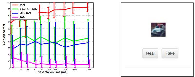
The LAPGAN paper contains a human evaluation experiment. Participants are given a series of images, and for each image asked whether they believe the image is real or generated. The image is chosen as random and could be either sampled from a GAN model, LAPGAN model, or the original dataset. The dataset used is CIFAR10 (consisting of ten classes of animals and automobiles). Prior to the experiment, the participants are given real images from the CIFAR10 dataset to look at. During the experiment, the participants are only presented each image for one of 11 durations ranging from 50ms to 2000ms. The experiment collects ~20k samples from the participants. Below (left) is a plot of the percentage of images classified as real with varying presentation times. The user-interface for this experiment is on the right.

The base GAN model is only able to fool the participants with $\leq$10% of the generated images. The LAPGAN and CC-LAPGAN (class-conditioned LAPGAN, where the class label is also given to the generative model) sport an impressive improvement, with around 40% generated images being real enough to fool humans. However, this is still a lot lower than the $>$90% rate for real images.

References

- ↑ 1.0 1.1 1.2 Goodfellow, Ian, et al. "Generative adversarial nets." Advances in Neural Information Processing Systems. 2014.
- ↑ 2.0 2.1 2.2 Denton, Emily L., Soumith Chintala, and Rob Fergus. "Deep Generative Image Models using a Laplacian Pyramid of Adversarial Networks." Advances in Neural Information Processing Systems. 2015.