Course:CPSC522/MCMC

Markov Chain Monte Carlo (MCMC)

MCMC is a class of Markov chain-based algorithms used to generate samples for use in Monte Carlo integration.

Principal Author: Ricky Chen
Collaborators: Jiahong Chen, Yan Zhao

Abstract

Monte Carlo Integration is briefly reviewed, and Markov Chain Monte Carlo is introduced as a method for solving Monte Carlo Integration when the samples are in high dimensions. We briefly review Monte Carlo Integration. Then we describe the theoretical justifications behind MCMC algorithms, and outline the generic Metropolis-Hastings algorithm and the commonly used Gibbs sampler.

Background

Knowledge of probability distributions, expectations, and basic properties of Markov chains are assumed.

Monte Carlo Integration

The goal of Monte Carlo integration is to approximate $E[f(X)]$ where $X$ is a possibly-multidimensional random variable from some target distribution $\pi$. Due to the definition of expectation, this means we can approximate any integral of the form

$E[f(X)]=\int f(x)\pi (x)dx$

Where $\pi$ satisfies the properties of a density function.

Example

Applied Monte Carlo integration on estimating the area of a unit circle. The red samples are within the circle and the blue samples are outside. The fraction of red samples is the ratio $\pi /4$

Suppose we want to find the area within the unit circle and denote this area by $K$. This can be written as an integral over the space $\Omega =[-1,1]\times [-1,1]$.

$K=\int _{\Omega }\mathbf {1} _{x^{2}+y^{2}\leq 1}d(x,y)$

Where $\mathbf {1} _{A}$ is the indicator function

$\mathbf {1} _{A}:={\begin{cases}1&{\text{if }}A{\text{ is true}}\\0&{\text{if }}A{\text{ if false}}\end{cases}}$

First we must transform this integral to the form that Monte Carlo integration can solve by introducing a random variable $(X,Y)$ that is uniform over the space $\Omega$. Notice that the area of $\Omega$ is

$\int _{\Omega }d(x,y)=4$

Thus the uniform variable $(X,Y)$ over $\Omega$ has density function $\pi (x,y)=1/4$. We can now write

$E[f(X,Y)]=\int _{\Omega }f(x,y)\pi (x,y)d(x,y)=(1/4)\int _{\Omega }f(x,y)d(x,y)=K/4$

Where we define $f(x,y):=\mathbf {1} _{x^{2}+x^{2}\leq 1}$.

The simplest Monte Carlo simulation involves sampling $N$ times from the distribution of $\pi$, computing the value of $f$ for each sample, and then averaging to approximate $E[f(X,Y)]$.

${\frac {1}{N}}\sum _{i=1}^{N}f(X_{i},Y_{i})\approx E[f(X,Y)]$

This Monte Carlo simulation written as a Matlab function:

   function [estimate] = simPi(N)
   f = @(x,y) x^2 + y^2 <= 1;
   sum = 0;
   for i=1:N 
       x = rand*2-1;
       y = rand*2-1;
       sum = sum + f(x,y);
   end
   estimate = 4*sum/N;

With a high enough $N$, we get a decent estimate of $K\approx \pi$ (the constant 3.1415...).

Monte Carlo Integration Based on Markov Chains

The example above only samples from uniform distributions. However, when the distribution of interest is hard to sample from using basic Monte Carlo methods, MCMC is useful if we don't know how to explicitly sample from the target distribution $\pi$. At its core, MCMC methods make use of the following property of Markov chains.

Law of Large Numbers for Markov Chains

Let $X_{n}$ be a Markov chain in ${\mathcal {X}}$.

Suppose $X_{n}$ is homogeneous, irreducible, and the stationary distribution exists, then for any function $f:{\mathcal {X}}\rightarrow \mathbb {R}$,

${\frac {1}{N}}\sum _{i=1}^{N}f(X_{n})\rightarrow E[f(X_{\infty })]$

Where $X_{\infty }\sim \pi$ is the stationary distribution of the Markov chain.

Thus we can perform Monte Carlo integration by designing a Markov chain such that the stationary distribution exists and is the target distribution $\pi$, then we can simulate the Markov chain to obtain "samples". The law of large numbers assures us that the estimator ${\frac {1}{N}}\sum _{i=1}^{N}f(X_{n})$ is consistent, ie reaches the exact value as $N$ goes to infinity.

Metropolis-Hastings (MH) Algorithm

Illustration of a MCMC method sampling from the target distribution (grey). We wish to obtain samples (blue) from this distribution. The green path indicates the transitions of the MCMC method. While the method starts off on the tail of the target distribution, it eventually gets to the area of high densities and randomly traverses the space.

We begin by describing the most general algorithm, which does not make any assumptions for $\pi$, other than that we can evaluate it pointwise. The Metropolis-Hastings algorithm often acts as a base for numerous other MCMC methods.

---

MH inputs:

1. A target distribution $\pi :{\mathcal {X}}\rightarrow \mathbb {R}$ that we can evaluate pointwise.

2. A proposal distribution/transition $q(x\rightarrow y)$ from which we can simulate $q(x\rightarrow \cdot ):{\mathcal {X}}\rightarrow \mathbb {R}$ and evaluate pointwise.

MH algorithm:

1. Initialize $x^{0}$ arbitrarily and set $F\leftarrow 0$

2. Loop $i=1,2,3,\dots ,N$ (until enough samples are generated):

(a) Propose a new state, $x'\sim q(x^{(i=1)}\rightarrow \cdot )$

(b) Compute

$A(x^{(i-1)}\rightarrow x')=\min \left\{1,{\frac {\pi (x')q(x'\rightarrow x^{(i-1)})}{\pi (x^{(i-1)})q(x^{(i-1)}\rightarrow x'))}}\right\}$

(c) Accept $x'$ as the new state $x^{(i)}$ with probability $A(x^{(i-1)}\rightarrow x')$; otherwise, accept $x^{(i-1)}$ as the new state.

(d) $F\leftarrow F+f(x^{(i)})$

3. Return $F/N$

---

The MH algorithm traverses the space of ${\mathcal {X}}$ where the step direction is proposed by $q(y|x)$ but the decision of whether to take the step is decided based on the acceptance ratio $A(x^{(i-1)}\rightarrow x')$. The acceptance ratio increases if the proposed state $x'$ is in a region with high density, and decreases if the proposed state is in a region of low density based. This makes sense intuitively since we would want more samples from a high density region.

Proof of Correctness

To prove that the MH algorithm does indeed simulate a Markov chain with stationary distribution $\pi$, we prove a stronger condition, the detailed balance equation which says for any $x,y\in {\mathcal {X}}$,

$\pi (x)p(x\rightarrow y)=\pi (y)p(y\rightarrow x)$

Where $p(x\rightarrow y)$ is the probability of transitioning from $x$ to $y$. The detailed balance equation implies that $\pi$ is the stationary distribution. To see this, simply take the sum over $x$ on both sides.

$\sum _{x}\pi (x)p(x\rightarrow y)=\sum (x)\pi (y)p(y\rightarrow x)\implies \sum _{x}\pi (x)p(x\rightarrow y)=\pi (y)$

Detailed balance is trivially true for $x=y$. First see that for $x\neq y$, the transition function is the probability of sampling $y$ at step 2(a) times the probability of acceptance

$p(x\rightarrow y)=q(y|x)A(x\rightarrow y)$

The proof of detailed balance for the MH algorithm is very simple:

$\pi (x)p(x\rightarrow y)=\pi (x)q(y|x)A(x\rightarrow y)$

$\pi (x)p(x\rightarrow y)=\min\{\pi (x)q(y|x),\pi (y)q(x|y)\}$

$\pi (x)p(x\rightarrow y)=\min\{\pi (y)q(x|y),\pi (x)q(y|x)\}$

$\pi (x)p(x\rightarrow y)=\pi (y)q(x|y)A(y\rightarrow x)$

$\pi (x)p(x\rightarrow y)=\pi (y)p(y\rightarrow x)$

Thus applying law of large numbers, we've proven the correctness of the MH algorithm. Similar proofs are constructed for other MCMC algorithms.

Notes

• The density $\pi$ always appears in a ratio, so we may use the MH algorithm even if we only know the density up to a normalizing constant $\pi =\pi ^{*}/Z$, where $Z>0$ is the normalization constant.

${\frac {\pi (x')}{\pi (x)}}={\frac {\pi ^{*}(x')/Z}{\pi ^{*}(x)/Z}}={\frac {\pi ^{*}(x')}{\pi ^{*}(x)}}$

• The acceptance step can be implemented by sampling from a Bernoulli distribution with probability $A(x^{(i-1)}\rightarrow x')$, or by sampling $U$ from a uniform distribution on (0,1) and checking if $U\leq A(x^{(i-1)}\rightarrow x')$
• From a practical perspective, it may be preferable to compute the acceptance ratio $A(x^{(i-1)}\rightarrow x')$ in log-space.

Example

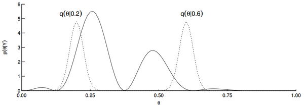
Suppose we have a posterior distribution of the form

$\pi (\theta |Y)\propto f(Y|\theta )\pi (\theta )$

With the distributions given by $Y=(Y_{1},Y_{2},\dots ,Y_{n}),\;Y_{i}|\theta \sim {\text{Bin}}(1,\theta )$ and $\pi (\theta )=2\cos ^{2}(4\pi \theta )$ This corresponds to having a binomial distributed likelihood and a non-conjugate prior, resulting in a posterior density that cannot be normalized or sampled from easily. Instead, we can use Metropolis-Hastings to sample from this target distribution. We will use a Normal proposal distribution centered around the current sample, meaning our proposals will be random walks, with length depending on $\sigma$, the standard deviation.

$q(\theta \rightarrow \theta ')\propto \exp \left\{{\frac {1}{2\sigma ^{2}}}(\theta -\theta ')^{2}\right\}$

Below is a plot of the posterior distribution and two examples of the proposal distribution if the current samples are 0.2 and 0.6. ($\sigma =0.1$)

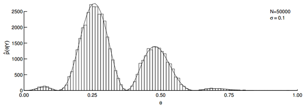
Using the Metropolis-Hastings algorithm with 50,000 samples and $\sigma =0.1$, we get the following histogram of samples.

As we can see, the histogram closely matches the target distribution.

Tuning the Proposal Distribution

Samples from a MCMC simulation over time based on three different random walk proposals. The top simulation has a good mixing rate. The middle simulation only proposes short walks, so the mixing rate is much lower. The bottom simulation often proposes states that are too far away, so the rejection rate is high; thus leading to a low mixing rate as well.

The tuning problem refers to how the choice of proposal distribution can change the outcome of the MCMC algorithm. The simplest proposal distribution is a random walk in any direction. Imagine a Gaussian distribution centered around the current point with a fixed covariance matrix. Then if the proposal distribution has a high variance, the Markov chain is more likely to jump around. If the proposal distribution has low variance, then the Markov chain may not move very much in the same number of iterations. On the other hand, if the variance is so high that it frequently proposes a point outside the current mode, then the rejection rate shoots up. This behavior is shown in the figure on the right, with sigma being the standard deviation of a Gaussian proposal distribution.

The proposal distribution should in some sense mimic the true distributions, so a slightly more clever proposal may be an approximation of the target $\pi$. Another property a proposal might have is that it may only update one variable at a time. For all these different choices we get a different transition operator, and any of these transition operators are valid in a MH algorithm.

In fact, we can mix and match transition operators and still have a valid MH algorithm, as long as the concatenation of the transition operators is still irreducible. This leads to what is known as the Gibbs sampler.

Gibbs Sampler

The Gibbs sampler is a special case of the MH algorithm where the transition proposals only change one variable at a time. Suppose the target distribution has $k$ dimensions $(X_{1},X_{2},\dots ,X_{k})\sim \pi$ and we knew the conditional probabilities

$q_{i}:=\mathbb {P} (X_{i}|X_{j}{\text{ for all }}i\neq j)$

Then we can alternate between the set of conditionals $\{q_{i}\}$ as the transition distribution. While each $q_{i}$ does not yield an irreducible Markov chain, the algorithm is valid as long as the concatenation $q_{1}q_{2}\dots q_{k}$ is irreducible.

---

Gibbs algorithm:

1. Initialize $x^{(0)}$ arbitrarily, $F\leftarrow 0$

2. Loop $i=1,2,3,\dots ,N$ (until enough samples are generated):

(a) $x^{(i)}\leftarrow x^{(i+1)}$

(b) Sample $M$ uniformly from $\{1,2,\dots ,k\}$

(c) Sample $x_{M}^{(i)}\sim \mathbb {P} (X_{M}|X_{j}{\text{ for all }}j\neq M)$

(d) $F\leftarrow F+f(x^{(i)})$

3. Return $F/N$

---

The Gibbs sampler can be more convenient than the basic MH algorithm, due to the avoidance of an accept-reject step. The acceptance ratio can be shown to always be 1. A common variant of the Gibbs sampler proposed here is to deterministically go through each dimension instead of sampling in step 2(b).

Of course, the main caveat of the Gibbs sampler is that knowledge of all the full conditional densities $q_{i}$ are required to be known, so this is a stronger condition than the basic MH algorithm.

Practical Concerns

Because MCMC algorithms all traverse the space using a Markov chain, the samples obtained are said to be correlated. While the law of large numbers does not assume any sort of low correlation or independence between samples, it is a theorem that only holds true as the number of samples goes to infinity. Since infinity is a concept that cannot be realized in any real application, some common hacks are used to improve the performance of MCMC algorithms.

Thinning

In order to break the dependence between samples, some have suggested to sample only once every $d$ transitions. This hack is known as thinning. Thinning is believed to help get more independent samples and also helps save memory as only a fraction of the samples are now stored. However, from a theoretic point of view, this hack is completely unnecessary as long as the chain is irreducible.

Burn-in

Since MCMC algorithms often randomly choose a point to start at, in high dimensions it is very likely this random initialization starts off at an area of low density. Then due to the Markov chain behavior, it may take some time before the MCMC algorithm reaches an area of high density. Oftentimes, the first few iterations are ignored (no samples are taken). This allows the Markov chain to traverse to an area of high density first before taking samples. This is known as having a burn-in interval.

Applications

MCMC can be applied in any context where the density of interest is too complex for simple sampling methods. For example, the Gibbs sampler is widely used in sampling from directed graphical models and the Ising model.

Also, MCMC are often used for calculating numerical approximations of multi-dimensional integrals, for example, Bayesian statistics, computational physics, computational biology and computational linguistics.

Annotated Bibliography

• Robert, Christian, and George Casella. Monte Carlo statistical methods. Springer Science & Business Media, 2013.
• Iain Murray. Monte Carlo Inference Methods. NIPS Tutorial 2015.
• Michael Eichler. Stat24600. University of Chicago.