Course:CPSC522/Exploring Results of Conditional Generative Adversarial Networks with Self-Organizing Maps

Exploring Results of Conditional Generative Adversarial Networks with Self-Organizing Maps

In this page we use Self-Organizing Maps to analyze the results of conditional Generative Adversarial Networks in the task of Image-to-Image translation.

Authors: Michela Minerva, Svetlana Sodol

Abstract

Conditional Generative Adversarial Networks (cGANs) are a specific type of Generative Adversarial Networks (GANs) and represent an example of conditional generative models. An important application area of cGANs is image-to-image translation. Self Organizing Maps (SOMs) are an unsupervised method that allows one to explore the topographical relationship of input data, and can be used as a clustering method. In this page, we perform image-to-image translation on 5 different image datasets. Then, we apply SOMs in order to obtain an insight on the generated results and on properties of the translation. We apply SOMs in settings specifically designed to conduct particular investigations. Our results indicate that the translation the cGAN performs does not preserve the similarity properties that SOM uses to cluster images. We also see differences in metrics and properties of the SOM results depending on the dataset, as we expected. We go on to outline the many future possibilities for extending this study.

Builds on

This page builds on concepts related to deep learning and unsupervised learning.

The method explained in this page uses Conditional GANs applied to the task of image-to-image translation. Conditional GANs are a specific type of Generative Adversarial Networks; Course:CPSC522/Generative Adversarial Networks is another page that focuses on GANs. Image-to-image translation is a class of problems in computer vision.

This method also uses Self-organizing maps, a type of unsupervised artificial neural networks.

Related Pages

Generative Adversarial Networks talks about GANs in general and focuses on an application of these architectures. Conditional GANs for image-to-image translation focuses on the application of GANs on image-to-image translation. Self-organizing maps are related to vector quantization methods; Self-organizing maps specifically talks about this topic in more detail.

Content

Introduction

In image-to-image translation, an input image from the source domain is translated into an output image in the target domain. This task can be formulated as a generative problem: the output image is synthesized using a generative model conditioned on the input image. GANs represent state-of-the-art methods to perform this domain transfer task. When training data consist of pairs of images from the two domains, this task takes the name of paired image-to-image translation. Conditional GANs are among the most used methods in this specific setting.

Self-Organizing Maps are a type of neural networks that can be applied to perform dimensionality reduction, and are trained using unsupervised learning. Similarly to vector quantization, once trained, a SOM associates an input sample to its representative node. We can view this process as a form of clustering, where samples associated to the same node belong to the same cluster. SOMs describe a mapping between the input space and a lower-dimensional map space, where nodes live. It is worth noting that SOMs preserve the topological properties of the input space. SOMs have been used for clustering and classification of visual data.

We still have little understandings on what a conditional GAN learns during the training process for paired image-to-image translation. The trained generative model performs a translation between the source and target domain. We want to explore whether some specific characteristics and structures get translated, and whether meaningful relationships between data in the source domain are maintained in the target domain. Exploring different datasets allows us to assess how much these properties vary depending on the datasets involved in the translation. We adopt SOM in order to perform this analysis. Hence, we will evaluate whether the translation performed by cGAN maintains the specific characteristics that SOM rely upon when exploring and grouping data. We will evaluate to which extent SOM can find the same structures and topographical relationships both in the source and the target domain containing generated fake data. We will also study the ability of SOM to distinguish between real and fake data within the output domain.

After a short background introduction on GANs and SOMs, this page illustrates the method and the evaluation used during tests and discusses the results.

Background

cGAN and image-to-image translation

Image-to-image translation is the task of transforming a given image into a corresponding output image. It can be viewed as a generative problem, where the output image is generated in a controlled way, conditioned by the input image. Conditional GANs are a powerful technique that allows one to solve problems in several applications of image-to-image translation.

Example of image-to-image translation obtained with cGAN during the tests, for the facade labels to photo dataset. From left to right: real image in the target domain, real image in the source domain, generated image in the target domain.

Conditional Generative Adversarial Networks (cGANs) are a specific type of Generative Adversarial Networks (GANs) in which the generation of data is performed in a conditional setting. The method for synthesizing data is similar to the one adopted in GANs, but the generation is conditioned on input data. The conditioning input data represents the source image for the translation, whereas the generated image is an image in the target domain. Current state-of-the-art image-to-image translation methods rely on cGANs, and their flexibility allows their use inside more complex frameworks. Moreover, cGANs can be trained on different data to perform translations between very different datasets without changing network architecture or loss function; in other words, they can be used for solving several different image-to-image translation problems.

For the investigations conducted in this page it is important to note that cGANs perform paired image to image translation. This differentiates cGANs from other types of GANs, such as cycleGANs, that perform unpaired image to image translation, and motivates our choice of choosing cGANs. In paired image-to-image translation, training and testing data are in form of couples of images from the source and target domains; for each image in the target domain there is a counterpart in the source domain and vice versa. On the other hand, in unpaired image translation images in the two domains have no correspondences.

For our page we use Pix2Pix, the first cGAN proposed for image-to-image translation. Code for this project is available in Pix2Pix and cycleGAN's GitHub repository, together with datasets and pretrained models. We use pre-trained models published by Pix2Pix's authors, one for each couple of domains, in order to generate our own test data. We also use test sets available on the same website.

Heat map for the facades_label2photo dataset. SOM was executed on a set with 50 fake images and 50 real images in the facade_photo domain. The map is the low-dimensional (2D) output space where nodes lie; each square represents a node. The color is a frequency representing the number of samples in the input space associated with that particular node.

SOM

A Self-Organizing Map is a method of dimensionality reduction. It can be thought of as creating a low-dimensional "map" of the distribution of input data living in a high-dimensional space. It is special, as this is done by initializing a structured low-dimensional map of random nodes, usually a 2D map, which have associated weight vectors in the input data space; this map is the low-dimensional space where resulting nodes lie. Then, each input sample is associated to one of the nodes, and simultaneously nodes are moved with each input sample to closer match it.

During the learning process, the closest node to each sample is titled its "winner" and can thus be used as its cluster label - inputs that share the same winner node can be seen as clustered together as they are similar. In this way a SOM can be interpreted as a clustering method.

One of the results that SOM produces is a heat map, i.e. a frequency map of the number of times each node has been a winner through all the input samples. See the image on the right for an example. The weights of the nodes in the resulting map are organized such that two input samples who have neighbouring winners are more alike than two input samples whose winners are further apart. This allows the SOM to preserve topological structure of the input data. For more details on the algorithm and applications see Self-Organizing Maps .

For our exploration we use the freely available SOM implementation in Python titled MiniSOM from https://github.com/JustGlowing/minisom.

Method

Image sets involved in our investigations and their relationships. The color of the set indicates the domain (Green: source, red: target), the contour of the set indicates the type of images (Solid line: real, dashed line: generated). Arrows indicate a one-to-one relationship between images in two domains, and the label details the relationship.

The method we test combines the use SOMs and GANs; it first uses a conditional GAN to perform image-to-image translation and generate fake images, then it applies SOMs to the results in order to discover meaningful groupings in the data. We apply SOMs to specific sets of data, and this allows us to perform specific investigations.  These investigations and the ways SOMs are applied to perform them are detailed in the following sections. Testing different datasets allows us to assess how these considerations change  across different datasets.

Analysis of real source data and fake target data: Translation

A conditional GAN performs paired image-to-image translation. It takes an input image from source domain $A$ and generates an image in target domain $B$. By running SOM on data before and after the translation we expect to obtain useful information regarding GAN's translation. In this step, we apply SOM separately on two sets: the set of real images in $A$, and the set of generated images in $B$.

We compare the results of these two SOMs. This allows us to study to which extent the grouping (or heat maps) generated by SOMs on a specific set of images changes before and after applying GAN’s translation. In other words, we study the similarity between clusters in real data and clusters in generated fake data. If the results of SOM do not change significantly, this might indicate that GAN’s translation maintains properties in images that SOMs rely upon for computing heatmaps. SOMs maintain topological properties of the input space when performing dimensionality reduction. Hence, if SOMs results are not largely different before and after GAN’s translation, we can say that the properties of the input space that are maintained by SOM when computing heat maps are also maintained by a cGAN when translating between the two domains. Vice versa, if results are significantly different, the translation performed by GAN affects properties in the data that are important for SOMs.

To perform this evaluation we use SOM as a clustering algorithm. This translates to the following idea: we count how many real images in domain $A$ are grouped together by SOM, and we determine how many of their synthesized counterparts in domain $B$ are clustered together again. In this way we assess to which extent the clustering changes between the two domains before and after the translation.

Analysis of real and fake target data: Fake detection

Another object of our study focuses on the use of cGAN as image-to-image translation tool specifically in the paired setting. We perform a single SOM on a set of images from the target domain $B$ that includes both real and synthesized fake images. By running SOM on this mixed data we expect to understand whether SOM can be used for discriminating between real and synthesized images, and how this property changes across different datasets. This can be evaluated by analyzing if images from the two categories tend to be grouped in separate clusters, or if they are mixed inside the clusters created by SOM.

Moreover, we exploit the property that the image translation performed by cGAN is paired. The test set, similarly to the training set, consists of couples of images from the two domains; in other words, there is a correspondence between each image in the source domain an one image in the target domain. Hence, we perform SOM on a set of images in the target domain $B$ where, for each real image in the source domain we have:

• The corresponding real image in the target domain
• The corresponding synthesized image in the target domain

This allows us to evaluate whether fake images are clustered together with real images in the target domain $B$ that correspond to the original image in the source domain $A$.

Experiments

This section provides details on the experiments conducted in order to perform investigations and illustrates the adopted metrics.

Datasets

We test our predictions on 5 datasets of images, all available in Pix2Pix and cycleGAN's GitHub repository. Each dataset is originally made up of 50 pairs of images in two different domains ($A$ and $B$). We used the 50 images from each of the source domains as inputs to a pre-trained cGAN for the specific domains. The cGAN additionally gave us 50 fake images in the target domain $B$ from corresponding inputs out of the 50 real images. Here are the datasets with their domains that we use:

• day2night: real image of a location during the day, real image of the location at night. The cGAN produces fake image of the location at night.
• edges2shoes: drawing of edges of a shoe, real image of the same shoe. The cGAN produces a fake image of the shoe.
• facades_label2photo: label map for the facade, real photo of the same facade. The cGAN produces a fake photo of the facade.
• map2sat: real aerial map, real satellite photo. The cGAN produces a fake satellite photo.
• sat2map: real satellite photo, real aerial map. The cGAN produces a fake aerial map.

Models

For each dataset we fit 4 SOM's:

1. Real images in domain A
2. Real images in domain B
3. Fake images in domain B (produced by cGAN)
4. All images of domain B

A simple detail of all the SOM maps that we collect is the number of non-empty clusters in the resulting map.

Jaccard similarity

Many of our evaluation metrics for comparison of clusterings are based on the Jaccard set similarity (or Jaccard index). In mathematical language it is equal to:

$J(S_{1},S_{2})={\frac {|S_{1}\cap S_{2}|}{|S_{1}\cup S_{2}|}}$

where $S_{1}$and $S_{2}$ are the two sets whose similarity we wish to calculate. This score will be a value between 0 and 1. Two sets who have all the same elements will have the perfect score of 1, and two sets who do not share any common elements will be given a score of 0. Thus, the closer this score is to 0, the less similar the two sets are.

In general, the expected value of the Jaccard similarity for two random sets approaches 1/3 as the size of sets approach infinity. A stretch of this interpretation could be that sets that have Jaccard similarity of larger than 1/3 are more similar than random, and sets with Jaccard similarity of less than 1/3 are less similar than random. Although, this is not to say that sets with Jaccard similarity of 0.4 are similar - they do share less than half of actual set members. It is dependent on the task of what is to be considered a cut off for two sets being titled "similar enough". What can be done with the Jaccard scores freely is saying that sets A and B with a Jaccard score of 0.3 are less similar than sets C and D with Jaccard score of 0.6.

In our experiments, sets are represented by clusters of images computed by SOMs. Hence, the Jaccard similarity is adopted as a metric to measure the similarity between these clusters. Next sections will discuss how Jaccard similarity is used as a metric in our investigations.

Translation metrics

For this metric we compare the SOM maps 1 and 3, when the fake and real images are processed separately. SOM 1 essentially maps the inputs to the cGAN and SOM 3 maps the outputs of the cGAN. This can give insight into how the translation preserves the topology of the inputs to cGAN in the outputs, if at all.

We do this by finding out the sets of all images for each cluster. Then, for each image we compare the set of images it was clustered with in the real domain to the set of images its fake counterpart was clustered with in the fake domain. This is done by Jaccard set similarity and then the mean and medians of this measure are reported for comparison between datasets.

Another set of set comparisons is performed by the cluster (not by image as the previous one). Each cluster's set of members is compared to all clusters in the other domain and the best match for each cluster is found by Jaccard set similarity. The mean and median of the Jaccard similarity for the best matches across all clusters are reported for comparison between datasets.

Fake detection metrics

For this metric we compare the SOM maps 2 and 3 when the fake and real images in the same domain are processed separately. This can give insight if the SOM finds the same structures in the fake dataset, produced by the cGAN, as in the real, that are the expected "ground truth" images (from which the inputs of the other domain were made from). We perform the same manipulations using Jaccard similarity by image and by cluster as described above.

Another metric for this part of the evaluation is an aggregated score of how many real images had preserved some members of their clusters from the real dataset to the fake. This is done by summing up the size of intersections between a cluster from SOM 2 and each of the clusters from SOM 3. Only intersections and clusters of more than 1 element are considered, as an image is always clustered with itself. This sum is reported along with the sizes of the clusters for comparisons between datasets. An aggregated score is calculated and reported as the total score over all clusters divided by the total number of elements in the clusters. The score is thus between 0 and 1, a score of 1 meaning that all images have similar co-cluster members in both SOMs.

The last two metrics we use are from the combined SOM 4. This can provide insight into if the SOM can tell apart the fake from the real image in the same pair as well as in general discriminate between the fakes and the reals. For the former we calculate the number of pairs for which both the fake and the real share the winner node. For the latter we report the number of clusters that are solely made up of real images only or of fake images only.

Results

Frequency heatmaps

Here is an example of the 4 frequency maps that result from SOM trained on different subsets of the cGAN datasets. The examples are for the day2night dataset. The frequency maps cannot be compared directly, as the rotation of the map could be permitted and thus resulting in node label permutation, but it is possible to see the local relationships between nodes and things like cluster number and size. Darker nodes mean more input samples to the SOM have that node as its winner. Nearby nodes are also local neighbours of each other in the input space.

• 

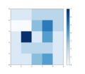  This is a frequency heatmap of SOM trained on the day2night dataset with 50 images of a location at night time. All of these images are faked by cGAN from real images of the same place at day time as inputs.

• 

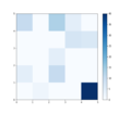  This is a frequency heatmap of SOM trained on the day2night dataset with 100 images, 50 of which are the real images and 50 are corresponding fake images of the same location at night time. The fake images are produced by cGAN from real images of the same place at day time as inputs.

• 

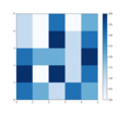  This is a frequency heatmap of SOM trained on the day2night dataset with 50 images of locations at day time.

• 

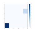  This is a frequency heatmap of SOM trained on the day2night dataset with 50 images of locations at night time.

Translation

dataset	clusters in real SOM	clusters in fake SOM	mean Jaccard for image	median Jaccard for image	mean Jaccard for cluster	median Jaccard for cluster
day2night	21	23	0.224	0.000	0.369	0.333
edges2shoes	22	22	0.251	0.000	0.399	0.292
facades_labels2photo	21	21	0.049	0.000	0.295	0.200
map2sat	23	22	0.028	0.000	0.264	0.143
sat2map	22	21	0.019	0.000	0.269	0.167

From the above results we can see that the SOMs created from the fake and from the real images in the same domains are pretty different, albeit having very close number of clusters formed. The Jaccard similarities for clusters are pretty low, with the Jaccard similarities by image even smaller. This indicates that it is possible that the cGAN has not preserved much of the overall structure of the distribution of the fake images that was present in the real images. I.e. the fakes of the cluster co-members of an image were not found to be cluster co-members of the fake image.

Fake detection

dataset	clusters in real SOM	clusters in fake SOM	mean Jaccard for image	median Jaccard for image	mean Jaccard for cluster	median Jaccard for cluster
day2night	2	23	0.046	0.025	0.212	0.212
edges2shoes	21	22	0.146	0.000	0.296	0.250
facades_labels2photo	21	21	0.032	0.000	0.358	0.200
map2sat	22	22	0.037	0.000	0.257	0.143
sat2map	22	21	0.074	0.000	0.321	0.250

Similar to the above, it looks like the SOM has not preserved much of the structure in the real vs fake of the same domain. The dataset that seems to perform a little better than others is the edges2shoes, especially on the mean Jaccard image measure for both translation and the fake detection metrics.

dataset	number of images with preserved cluster members by cluster	sizes of clusters	score
day2night	[26, 3]	[40, 10]	0.580
edges2shoes	[0, 0, 0, 0, 0, 2, 0, 6, 7, 0, 2, 0, 2, 0, 0, 0, 0, 0, 0, 0, 0]	[4, 1, 2, 4, 1, 2, 2, 9, 7, 1, 2, 1, 3, 1, 2, 1, 2, 1, 2, 1, 1]	0.473
facades_labels2photo	[0, 2, 0, 0, 0, 2, 0, 0, 7, 0, 2, 0, 0, 0, 0, 0, 0, 0, 0, 0, 0]	[2. 5. 1. 1. 1. 6. 1. 5. 8. 1. 5. 4. 2. 1. 1. 1. 1. 1. 1. 1. 1.]	0.351
map2sat	[0, 2, 3, 0, 0, 4, 0, 0, 0, 0, 0, 0, 0, 0, 0, 0, 0, 0, 0, 0, 0, 0]	[ 1. 5. 10. 7. 1. 8. 1. 1. 1. 1. 2. 1. 2. 1. 1. 1. 1. 1. 1. 1. 1. 1.]	0.265
sat2map	[0, 4, 8, 2, 0, 0, 0, 3, 0, 0, 0, 0, 0, 0, 0, 0, 0, 0, 0, 0, 0, 0]	[ 2. 6. 14. 3. 1. 1. 2. 5. 1. 1. 1. 1. 1. 1. 1. 1. 2. 2. 1. 1. 1. 1.]	0.472

Looking at this other metric, the scores are also pretty low, the largest score is for the day2night dataset. This dataset however has only 2 clusters in the real SOM in domain B which could be playing heavily into how the images are clustered, and thus are more likely to have the same co-cluster members. Since this metric sums over all of the fake clusters to compute the score, it could be the case that only the local relationships between images are preserved, which results in high score of this metric, but is not picked up by the Jaccard similarity measures.

dataset	clusters in combined SOM	pairs clustered together	fake only clusters	real only clusters
day2night	10	0	8	2
edges2shoes	22	27	3	5
facades_labels2photo	25	11	4	8
map2sat	24	15	9	7
sat2map	25	0	8	15

As would be expected based on the other measures, edges2shoes is the worst dataset for distinction between fake and real images, as it has most number of pairs clustered together. Judging by this metric, the sat2map dataset has the best fake detection of the 5 and its scores are mostly comparable to the top scores on other measures above too (albeit still not too great), discounting the score of the day2night due to its onle having 2 clusters and thus skewing results. It is interesting to note that the opposite dataset map2sat does not seem to bahave in a similar way.

The day2night dataset showcases complete separation of not only all pairs of fake and real images but also complete separation of clusters for fake and real images. However, the real dataset of day2night only has 2 clusters, which makes this a very biased dataset. The 2 real only clusters of the combined SOM are likely to be the same ones as the real only SOM has.

Follow up

To have some background to the interpretation of the Jaccard similarities we ran a follow up Jaccard similarity comparison set on the two real SOM maps 1 and 2. These are essentially the two parts of the datasets that were used in the training of the cGAN. The results of these are very consistent for the 5 datasets, with all the values reported in narrow ranges as follows:

• mean Jaccard similarity for images: 0.024-0.06
• median Jaccard similarity for images: 0.0-0.025
• mean Jaccard similarity for clusters: 0.2 - 0.35
• median Jaccard similarity for clusters: 0.18-0.2

It could be the case that the translaton of cGAN does not preserve the structure of the real images when creating the fake images, as was tested in the Translation part of our setup. It might instead preserve the comparative structure of the two subsets it was trained on (real A and real B images - what we have compared in the follow up) and then replicate that structure in what paired dataset it results in (real A (input) and fake B images (output) - this is the original Translation comparison) - as if it is trying to copy the cluster structure of the A to B relationship. This could provide an alternative interpretation to the low Jaccard similarity metrics in our Translation setup - if these numbers are the same in the follow up, then the cGAN did its job at picking out the relationship between the two image domains A and B and was able to use it (to an extent) when creating the fake B images. However, when comparing the follow up numbers to the Translation numbers, the results are all over, with some numbers matching, some being much larger and some being smaller. This essentially creates more questons than insights and warrants more research.

Discussion

Results for the translation experiment show that the grouping generated by SOMs on a dataset before and after GAN’s translation changes significantly. This suggests that elements in data that SOMs rely upon when computing results are affected by GAN’s translation. Moreover, this indicates that the translation does not maintain properties in the data space that SOMs maintain in the low-dimensional space produced by dimensionality reduction.

Analyzing results from the fake detection experiments, in particular the comparison of SOMs’ clustering for real and fake data in the target domain, when processed separately, we can observe a consistent behaviour. SOMs clustering is significantly different for real and fake images on the same domain.

According to the results of the fake detection experiment for the SOM on the mixed dataset, SOMs do not generally perform well in the task of discriminating real and generated images in one domain. This result is not surprising since this is not a trivial task. It is worth noting that the performance significantly changes depending on the dataset. In edges2shoes and facades_labels2photo more than half of the clusters contain mixed images; on the other hand in day2night and sat2map, where most of the clusters are real-only or fake-only, SOMs are able to distinguish the two categories. The amount of pairs clustered together also depends heavily on the dataset.

Future works

Our exploration leaves multiple questions unanswered and has a lot of variables still unaccounted for. If further explorations of using SOM with cGAN are successful, this could indicate that SOM is a good candidate to attempt to use for detection of fake images that exist out there in the internet or perhaps for detecting fakes in other domains.

The set of metrics used in the experiments is quite limited and very simple. More detailed considerations of the comparisons between clustering would provide more reliable results. Exploring the actual weight vectors of the winner nodes found in SOMs is one direction to take. Moreover, the size of our test sets is limited to 50 pairs of images each; it would be interesting to see if this trend of results extrapolates to datasets of the same domains but with larger size. The actual datasets that we used were limited by the available pre-trained cGAN models; a more detailed exploration of how this type of evaluation behaves with more types of images created by cGAN would be required.

A more detailed exploration of what exact images are getting paired together in the map2sat dataset SOM 4 might provide insights into what kind of similarity SOM is able to find in image data treated in this way, as opposed to other datasets.

There are many points of finetuning for the SOM models that could be used for such a task. The SOM that we fitted were all 5X5 2D maps, that start with random input samples as the weights. It might be more reliable to use the same initial weights for all the SOM's that are compared, such as initializing the map uniformly. A larger SOM might produce more fine-grained results, although for a dataset this size (50 pairs) the 25-node map had an okay balance, as it was able to find some groupings in the images.

Conclusion

In conclusion, in this page we combined the application of SOMs and GANs. We used SOMs in order to analyze properties of GANs’ translation, and we tested SOM clustering’s abilities to separate real and fake images. It was interesting to see SOMs work with image data treated as arrays of pixels rather than with feature representations such as SIFT bag of words. SOMs found different clustering before and after GANs translation, and they generally did not have a good performance in separating real and fake images. Although our experiments led us to some discoveries, there are still several questions to answer. Multiple possible future works can be carried out in order to fully exploit the potential of these methods.

To Add

Put links and content here to be added. This does not need to be organized, and will not be graded as part of the page. If you find something that might be useful for a page, feel free to put it here.