Course:CPSC522/Diffusion Probabilistic Model

Title

This page focuses on Diffusion Probabilistic Models, covering their introduction in Deep Unsupervised Learning using Nonequilibrium Thermodynamics, as well as a newer advancement, Denoising Diffusion Probabilisitic Models

Principal Author:Matthew Niedoba

Abstract

Generative models are a powerful class of models which are able to draw novel samples which match the distribution of their training distribution. One such class of generative models are diffusion probabilisitic models. These models consist of a forward trajectory which iteratively adds noise to the source data distribution to shift it towards a tractable prior. The reverse trajectory aims to model the reverse of this process, slowly shifting the distribution from the tractable prior back to the target data distribution.

Builds on

The forward and reverse trajectories of diffusion probabilisitc models are examples of Markov Chains. The models are optimized using the ELBO, a technique from Variational Inference.

Related Pages

Diffusion models are generative models. Other members of that class of model are Generative Adversarial Networks ,Variational Auto-Encoders, and Variational Recurrent Neural Networks.

Diffusion Probabilistic Models

Figure 1. A toy Swiss Roll distribution fit using diffusion probabilistic model. Top: The forward trajectory, starting from the base distribution on the left. Middle: Samples from the reverse trajectory. Bottom: Vector field showing the difference in estimated posterior mean from timestep $t$ to timestep $t-1$.

In Deep Unsupervised Learning using Nonequilibrium Thermodynamics, the authors introduce diffusion probabilistic models. This section summarizes the contributions of this paper, detailing the forward trajectory, reverse trajectory, training objective and experimental results.

Forward Trajectory

We define the distribution of our data as ${\textstyle q\left(\mathbf {x^{(0)}} \right)}$. Generally, this distribution, such as CIFAR-10 images is highly complex and intractable. New samples cannot be drawn from the data set directly. The forward trajectory is the process of converting this complex distribution into an analytically tractable distribution $\pi \left(\mathbf {y} \right)$ from which samples may be drawn, such as a multivariate Gaussian. The data distribution is transformed by iteratively applying a Markov diffusion kernel ${\textstyle q\left(\mathbf {x^{(t)}} |\mathbf {x^{(t-1)}} \right)=T_{\pi }\left(\mathbf {y} |\mathbf {y'} ;\beta _{t}\right)}$ where $\beta _{t}$ is the diffusion rate at time t. Two possible choices of kernel are Gaussian and Binomial, corresponding to

$$q\left(\mathbf {x^{(t)}} |\mathbf {x^{(t-1)}} \right)={\mathcal {N}}\left(\mathbf {x^{(t)}} ;{\sqrt {1-\beta _{t}}}\mathbf {x^{(t-1)}} ,\beta _{t}\mathbf {I} \right)$$

$$q\left(\mathbf {x^{(t)}} |\mathbf {x^{(t-1)}} \right)={\mathcal {B}}\left(\mathbf {x^{(t)}} ;\left(1-\beta _{t}\right)\mathbf {x^{(t-1)}} +{\frac {1}{2}}\beta _{t}\right)$$

Repeatedly applying the kernel, we obtain the forward trajectory

$$q\left(\mathbf {x^{(0\ldots T)}} \right)=q\left(\mathbf {x^{(0)}} \right)\prod _{i=1}^{T}q\left(\mathbf {x^{(t)}} |\mathbf {x^{(t-1)}} \right)$$

Reverse Trajectory

To generate samples from the diffusion model, a model is trained to reverse the forward trajectory.

$$p\left(\mathbf {x^{(T)}} \right)=\pi \left(\mathbf {x^{(T)}} \right)$$

$$p\left(\mathbf {x^{(0\ldots T)}} \right)=p\left(\mathbf {x^{(0)}} \right)\prod _{i=1}^{T}p\left(\mathbf {x^{(t-1)}} |\mathbf {x^{(t)}} \right)$$

If $\beta _{t}$ is small, then the form of ${\textstyle p\left(\mathbf {x^{(t-1)}} |\mathbf {x^{(t)}} \right)}$will match ${\textstyle q\left(\mathbf {x^{(t)}} |\mathbf {x^{(t-1)}} \right)}$. That is, Gaussian transitions in the forward process will lead to Gaussian transitions in the reverse process. For Gaussian forward trajectories, the reverse trajectory is estimated by learning functions ${\textstyle \mu _{\theta }\left(\mathbf {x^{(t)}} ,t\right)}$and ${\textstyle \Sigma _{\theta }\left(\mathbf {x^{(t)}} ,t\right)}$which estimate the mean and covariance of the reverse trajectory transitions.

Training Objective

The objective in training is to maximize the log likelihood of the data

$${\mathcal {L}}=\int d\mathbf {x^{(0)}} q\left(\mathbf {x} ^{(0)}\right)log\ p\left(\mathbf {x} ^{(0)}\right)$$

Naively, ${\textstyle log\ p\left(\mathbf {x} ^{(0)}\right)}$ is intractable as it involves evaluating the integral

$$p\left(\mathbf {x} ^{(0)}\right)=\int d\mathbf {x} ^{(0\ldots T)}p\left(\mathbf {x} ^{(0\ldots T)}\right)$$

However, the authors transform this integral into an average over forward trajectory samples by multiplying top and bottom by ${\textstyle q\left(\mathbf {x} ^{(1\ldots T)}|\mathbf {x} ^{(0)}\right)}$

$$p\left(\mathbf {x} ^{(0)}\right)=\int d\mathbf {x} ^{(0\ldots T)}p(\mathbf {x} ^{(0\ldots T)})\cdot {\frac {q(\mathbf {x} ^{(1\ldots T)}|\mathbf {x} ^{(0)}))}{q(\mathbf {x} ^{(1\ldots T)}|\mathbf {x} ^{(0)}))}}$$

$$p\left(\mathbf {x} ^{(0)}\right)=\int d\mathbf {x} ^{(0\ldots T)}q(\mathbf {x} ^{(1\ldots T)}|\mathbf {x} ^{(0)}))\cdot {\frac {p(\mathbf {x} ^{(0\ldots T)})}{q(\mathbf {x} ^{(1\ldots T)}|\mathbf {x} ^{(0)}))}}$$

$$p\left(\mathbf {x} ^{(0)}\right)=\int d\mathbf {x} ^{(0\ldots T)}q(\mathbf {x} ^{(1\ldots T)}|\mathbf {x} ^{(0)}))\cdot {\frac {p(\mathbf {x} ^{(T)})\cdot p(\mathbf {x} ^{(T-1)})|\mathbf {x} ^{(T)})\cdots p(\mathbf {x} ^{(0)})|\mathbf {x} ^{(1)})}{q(\mathbf {x} ^{(T)}|\mathbf {x} ^{(T-1)}))\cdots q(\mathbf {x} ^{(1)}|\mathbf {x} ^{(0)}))}}$$

$$p\left(\mathbf {x} ^{(0)}\right)=\int d\mathbf {x} ^{(1\ldots T)}q\left(\mathbf {x} ^{(1\ldots T)}|\mathbf {x} ^{(0)}\right)\cdot p\left(\mathbf {x} ^{(T)}\right)\prod _{t=1}^{T}{\frac {p\left(\mathbf {x} ^{(t-1)}|\mathbf {x} ^{(t)}\right)}{q\left(\mathbf {x} ^{(t)}|\mathbf {x} ^{(t-1)}\right)}}$$

Although somewhat verbose, we can see that $p(\mathbf {x} ^{(0)})$ is now in the form of an expectation over samples from the forward trajectory $q(\mathbf {x} ^{(0\ldots ,T)}|\mathbf {x} ^{(0)})$. We can therefore produce sample based estimates of this value. Applying the modified form of $p(\mathbf {x} ^{(0)})$ to the Loss Equation produces

$${\mathcal {L}}=\int d\mathbf {x^{(0)}} q\left(\mathbf {x} ^{(0)}\right)log\left[\ \int d\mathbf {x} ^{(1\ldots T)}q\left(\mathbf {x} ^{(1\ldots T)}|\mathbf {x} ^{(0)}\right)\cdot p\left(\mathbf {x} ^{(T)}\right)\prod _{i=1}^{T}{\frac {p\left(\mathbf {x} ^{(t-1)}|\mathbf {x} ^{(t)}\right)}{q\left(\mathbf {x} ^{(t)}|\mathbf {x} ^{(t-1)}\right)}}\right]$$

Jensen's Inequality states that for a convex function $\varphi$, $\varphi \left(\mathbf {E} \left[\mathbf {X} \right]\right)\leq \mathbf {E} \left[\varphi \left(\mathbf {X} \right)\right]$. Noting that $\log(x)$ is convex, and that our expression for $p(\mathbf {x} ^{(0)})$ is in the form of an expectation, the evidence can be lower bounded as is typical in other variational inference methods. This method of lower bounding the log likelihood is known as the ELBO (Evidence Lower Bound).

$${\mathcal {L}}\geq L=\int d\mathbf {x} ^{(0\ldots T)}q\left(\mathbf {x} ^{(0\ldots T)}\right)\cdot log\left[p\left(\mathbf {x} ^{(T)}\right)\prod _{i=1}^{T}{\frac {p\left(\mathbf {x} ^{(t-1)}|\mathbf {x} ^{(t)}\right)}{q\left(\mathbf {x} ^{(t)}|\mathbf {x} ^{(t-1)}\right)}}\right]$$

$$L=\mathbb {E} _{\mathbf {x} ^{(0\ldots T)}\sim q}\left[\log {\frac {p\left(\mathbf {x} ^{(0\ldots T)}\right)}{q\left(\mathbf {x} ^{(1\ldots T)}|\mathbf {x} ^{(0)}\right)}}\right]$$

The loss is now in the form of an expectation over samples from the forward trajectory. However, it can be reformulated into an expectation into a sum of KL divergence and entropy terms which is advantageous because they are available in closed form for Gaussian probabilities. The full simplification is described in the Appendix of , but a condensed version, found in the appendix of is shown here for clarity. Although it is not important to know the exact steps to arrive at the simplified loss, this form of the loss functions is the jumping off point for the advances made in Denoising Diffusion Probabilistic Models.

$$L=\mathbb {E} _{\mathbf {x} ^{(0\ldots T)}\sim q}\left[\log {\frac {p\left(\mathbf {x} ^{(0\ldots T)}\right)}{q\left(\mathbf {x} ^{(1\ldots T)}|\mathbf {x} ^{(0)}\right)}}\right]$$

$$=\mathbb {E} _{\mathbf {x} ^{(0\ldots T)}\sim q}\left[\log p\left(\mathbf {x} ^{(T)}\right)+\sum _{t=1}^{T}\log {\frac {p\left(\mathbf {x} ^{(t-1)}|\mathbf {x} ^{(t)}\right)}{q\left(\mathbf {x} ^{(t)}|\mathbf {x} ^{(t-1)}\right)}}\right]$$

$$=\mathbb {E} _{\mathbf {x} ^{(0\ldots T)}\sim q}\left[\log p\left(\mathbf {x} ^{(T)}\right)+\log {\frac {p\left(\mathbf {x} ^{(0)}|\mathbf {x} ^{(1)}\right)}{q\left(\mathbf {x} ^{(1)}|\mathbf {x} ^{(0)}\right)}}+\sum _{t=2}^{T}\log {\frac {p\left(\mathbf {x} ^{(t-1)}|\mathbf {x} ^{(t)}\right)}{q\left(\mathbf {x} ^{(t)}|\mathbf {x} ^{(t-1)}\right)}}\right]$$

$$=\mathbb {E} _{\mathbf {x} ^{(0\ldots T)}\sim q}\left[\log p\left(\mathbf {x} ^{(T)}\right)+\log {\frac {p\left(\mathbf {x} ^{(0)}|\mathbf {x} ^{(1)}\right)}{q\left(\mathbf {x} ^{(1)}|\mathbf {x} ^{(0)}\right)}}+\sum _{t=2}^{T}\log {\frac {p\left(\mathbf {x} ^{(t-1)}|\mathbf {x} ^{(t)}\right)}{q\left(\mathbf {x} ^{(t-1)}|\mathbf {x} ^{(t)},\mathbf {x} ^{(0)}\right)}}\cdot {\frac {q\left(\mathbf {x} ^{(t-1)}|\mathbf {x} ^{(0)}\right)}{q\left(\mathbf {x} ^{(t)}|\mathbf {x} ^{(0)}\right)}}\right]\quad {\text{by Bayes Rule}}$$

$$=\mathbb {E} _{\mathbf {x} ^{(0\ldots T)}\sim q}\left[\log {\frac {p\left(\mathbf {x} ^{(T)}\right)}{q\left(\mathbf {x} ^{(T)}|\mathbf {x} ^{(0)}\right)}}+\log p\left(\mathbf {x} ^{(0)}|\mathbf {x} ^{(1)}\right)+\sum _{t=2}^{T}\log {\frac {p\left(\mathbf {x} ^{(t-1)}|\mathbf {x} ^{(t)}\right)}{q\left(\mathbf {x} ^{(t-1)}|\mathbf {x} ^{(t)},\mathbf {x} ^{(0)}\right)}}\right]$$

$$=\mathbb {E} _{\mathbf {x} ^{(0\ldots T)}\sim q}\left[-D_{KL}\left(q\left(\mathbf {x} ^{(T)}|\mathbf {x} ^{(0)}\right)||p\left(\mathbf {x} ^{(T)}\right)\right)+\log p\left(\mathbf {x} ^{(0)}|\mathbf {x} ^{(1)}\right)-\sum _{t=2}^{T}D_{KL}\left(q\left(\mathbf {x} ^{(t-1)}|\mathbf {x} ^{(t)},\mathbf {x} ^{(0)}\right)||p\left(\mathbf {x} ^{(t-1)}|\mathbf {x} ^{(t)}\right)\right)\right]$$

This loss is made up of two KL divergence terms and a cross entropy. Note that in the original derivation, the authors replace ${\textstyle -D_{KL}\left(q\left(\mathbf {x} ^{(T)}|\mathbf {x} ^{(0)}\right)||p\left(\mathbf {x} ^{(T)}\right)\right)}$ with the cross entropy minus the entropy which is equivalent.

Learning Beta

One key difference between this first paper and future diffusion probabilistic models is that the authors choose to learn the variance schedule of the forward trajectory $\beta _{t}$. The authors set $\beta _{1}$ to a small value, but otherwise optimize $\beta _{2,\ldots ,T}$ through gradient ascent on the learning objective.

Experimental Results

Figure 2. Diffusion probabilistic models applied to CIFAR-10. (a) Examples from the CIFAR-10 dataset. (b) Forward trajectory samples of the CIFAR-10 Examples. (c) Diffusion probabilistic model samples corresponding to the CIFAR-10 samples. (d) Unconditioned samples from the diffusion probabilistic model.

The authors demonstrated the effectiveness of their method by fitting a Diffusion Probabilistic Model to a toy 2D distribution, a binary heartbeat distribution and a variety of image datasets

Toy Example Results

The authors use a proof of concept "Swiss Roll" distribution to validate that diffusion models are capable of learning complex 2D distributions. For this problem, a Gaussian forward and reverse trajectory were used. Figure 1 shows that the reverse trajectory is capable of closely matching the target distribution for this simple problem.

Binary Heartbeat Distribution

To illustrate that diffusion probabilistic models can be used to capture binary distributions, the authors fit a model to a synthetic heartbeat dataset. The heartbeat dataset consists of sequences of 20 binary variables, with ones every 5th step and zeros elsewhere. The diffusion probabilistic model was able to almost perfectly match the synthetic distribution.

Image Datasets

The authors trained their method on a variety of image datasets, including MNIST digits, CIFAR-10, and Dead Leaf Images . They parameterize their reverse trajectory $\mu _{\theta }$ and $\mu _{\Sigma }$ using a multi-scale convolutional neural network. On MNIST, they claim superior performance as measured by a sample based estimate of the negative log likelihoods. When compared to other generative models, their method trails only generative adversarial networks.

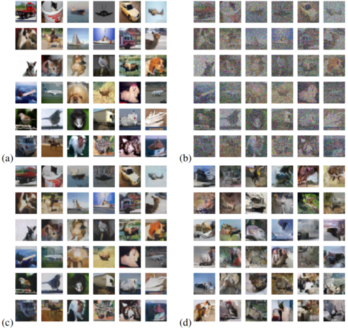
On CIFAR-10, they show qualitative samples highlighting that the model is able to produce reasonable samples from the data distribution. These samples are shown in Figure 2. Examining the samples from Figure 2c, we can see that the samples somewhat match the original dataset images, but contain some artifacts such as blurring and brightness shift. The samples in Figure 2d do not seem to correspond to any of the 10 classes and are not easily recognizable.

Conclusion

In this first paper, the authors introduce a new class of generative models and demonstrate its effectiveness through several experiments. Although the model performs well on the toy Swiss Roll problem and MNIST, the CIFAR-10 samples show clear room for improvement.

Denoising Diffusion Probabilistic Models

Figure 3. DDPM CIFAR10 unconditional samples

In the first paper, the authors introduced diffusion probabilistic models, and showed that they can generate image samples from various datasets including CIFAR10. However, the resulting sample quality is somewhat poor, especially in unconditional samples. In Denoising Diffusion Probabilistic Models, the authors seek to improve the quality of these samples. The authors select a specific parameterization of the forward and reverse process, which is guided by a connection between diffusion probabalistic models and denoising score matching. This section covers the modifications made to the previously introduced diffusion probabilistic model, and the experimental results reported in the work.

We follow the structure of the paper, covering the modifications made in the context of the three main terms of the training loss introduced previously

$$L=\mathbb {E} _{q}\left[L_{T}+\sum _{t>1}L_{t-1}+L_{0}\right]$$

$$L_{T}=D_{KL}\left(q\left(\mathbf {x} _{T}|\mathbf {x} _{0}\right)||\ p\left(\mathbf {x} _{T}\right)\right)$$

$$L_{t-1}=D_{KL}\left(q\left(\mathbf {x} _{t-1}|\mathbf {x} _{t},\mathbf {x} _{0}\right)||\ p_{\theta }\left(\mathbf {x} _{t-1}|\mathbf {x} _{t}\right)\right)$$

$$L_{0}=-logp_{\theta }\left(\mathbf {x} _{0}|\mathbf {x} _{1}\right)$$

Forward Trajectory and $L_{T}$

Unlike the previous paper, the authors decide here to fix the forward trajectory by setting a linear schedule for $\beta$. By fixing the diffusion rate, the loss term $L_{T}$ is constant since $q(\mathbf {x} ^{(T)}|\mathbf {x} ^{(0)})$ is fixed and $p(\mathbf {x} ^{(T)})={\mathcal {N}}\left(0,\mathbf {I} \right)$.

Reverse Trajectory and $L_{t-1}$

Next, the authors select the parameterization ${\textstyle p_{\theta }\left(\mathbf {x} ^{(t-1)}|\mathbf {x} ^{(t)}\right)={\mathcal {N}}\left(\mathbf {x} ^{(t-1)};\mu _{\theta }\left(\mathbf {x} ^{(t)},t\right),\beta _{t}\mathbf {I} \right)}$ where like in , ${\textstyle \mu _{\theta }\left(\mathbf {x^{(t)}} ,t\right)}$ is a neural network which outputs the mean of the distribution. The key difference between this parameterization and the parameterization used in is the covariance. Unlike , the authors here use a diagonal covariance matrix instead of a full covariance matrix. Further, they do not estimate the covariance at each timestep. Instead, they fix the scale of the variance to match the diffusion rate at every timestep.

The authors then use this parameterization to simplify $L_{t-1}$. Given $q\left(\mathbf {x} ^{(t-1)}|\mathbf {x} ^{(t)},\mathbf {x} ^{(0)}\right)={\mathcal {N}}\left(\mathbf {x} ^{(t-1)};{\tilde {\mu }}_{t}\left(\mathbf {x} ^{(t)},\mathbf {x} ^{(0)}\right),\beta _{t}\mathbf {I} \right)$, where ${\tilde {\mathbf {\mu } }}_{t}\left(\mathbf {x} ^{(t)},\mathbf {x} ^{(0)}\right):={\frac {{\sqrt {{\bar {\alpha }}_{t-1}}}\beta _{t}}{1-{\bar {\alpha }}_{t}}}\mathbf {x} ^{(0)}+{\frac {{\sqrt {1-\beta _{t}}}(1-{\bar {\alpha }}_{t-1})}{1-{\bar {\alpha }}_{t}}}\mathbf {x} ^{(t)}$ is the posterior mean of the forward trajectory, the KL divergence can be rewritten as

$$L_{t-1}={\frac {1}{2\beta _{t}^{2}}}||{\tilde {\mathbf {\mu } }}_{t}\left(\mathbf {x} ^{(t)},\mathbf {x} ^{(0)}\right)-\mathbf {\mu } _{\theta }\left(\mathbf {x} ^{(t)},t\right)||^{2}+C$$

Where C is a constant with respect to the parameters of the reverse trajectory. From this loss formulation it is clear that to minimize $L_{t-1}$, the mean of the reverse trajectory must match the posterior mean of the forward trajectory. Since the posterior mean of the forward trajectory can be computed in closed form given $\mathbf {x} ^{(t)}$ and $\mathbf {x} ^{(0)}$, $\mathbf {\mu } _{\theta }$ can therefore be optimized using this L2 error over random samples from $q(\mathbf {x} _{t},\mathbf {x_{0}} )$.

Inspired by , the authors provide an alternate objective which relates the parameterization of the reverse trajectory to a score matching objective over varying noise scales. Since the forward trajectory is a Markov chain with Gaussian transitions, we can sample $\mathbf {x} ^{(t)}$ from the forward trajectory using the reparameterization trick ie: $\mathbf {x} _{t}\left(\mathbf {x} _{0},\mathbf {\epsilon } \right)=\mu +\sigma \mathbf {\epsilon }$, $\mathbf {\epsilon } \sim {\mathcal {N}}\left(\mathbf {0} ,\mathbf {I} \right)$. For the Gaussian forward trajectory which is specified as $q(\mathbf {x} ^{(t)}|\mathbf {x} ^{(t-1)})={\mathcal {N}}\left(\mathbf {x} ^{(t)};{\sqrt {1-\beta _{t}}}\mathbf {x} ^{(t-1)},\beta _{t}\mathbf {I} \right)$, we have $\mathbf {x} _{t}\left(\mathbf {x} _{0},\mathbf {\epsilon } \right)={\sqrt {{\bar {\alpha }}_{t}}}\mathbf {x} _{0}+{\sqrt {1-{\bar {\alpha }}_{t}}}\mathbf {\epsilon }$ where ${\textstyle {\bar {\alpha }}_{t}=\prod _{i=1}^{t}(1-\beta _{t})}$. By substituting this function of $\mathbf {x} _{t}$ into the ${\tilde {\mathbf {\mu } }}_{t}\left(\mathbf {x} ^{(t)},\mathbf {x} ^{(0)}\right)$ of $L_{t-1}$ equation, expanding, and rearranging for $\mu _{\theta }$, the authors find that an optimal choice of parameterization for $\mathbf {\mu } _{\theta }$ is

$$\mathbf {\mu } _{\theta }\left(\mathbf {x} ^{(t)},t\right)={\frac {1}{\sqrt {1-\beta _{t}}}}\left(\mathbf {x} ^{(t)}-{\frac {\beta _{t}}{\sqrt {1-{\bar {\alpha }}_{t}}}}\mathbf {\epsilon } _{\theta }\left(\mathbf {x} ^{(t)},t\right)\right)$$

Where $\mathbf {\epsilon } _{\theta }(\mathbf {x} ^{(t)},t)$ is a function approximator which estimates the noise used to generate $\mathbf {x} ^{(t)}$. Substitution this parameterization of $\mathbf {\mu } _{\theta }$, $L_{t-1}$ simplifies to

$$L_{t-1}=\mathbb {E} _{x_{0},\epsilon }\left[{\frac {1}{2\beta _{t}(1-\beta _{t})}}||\mathbf {\epsilon } -\mathbf {\epsilon } _{\theta }\left({\sqrt {{\bar {\alpha }}_{t}}}\mathbf {x} _{0}+{\sqrt {1-{\bar {\alpha }}_{t}}}\mathbf {\epsilon } ,t\right)||^{2}\right]$$

The authors empirically find that the coefficient impedes sample quality, so they train their model using a simplified objective:

$$L_{simple}=\mathbb {E} _{x_{0},\epsilon ,t}\left[||\mathbf {\epsilon } -\mathbf {\epsilon } _{\theta }\left({\sqrt {{\bar {\alpha }}_{t}}}\mathbf {x} _{0}+{\sqrt {1-{\bar {\alpha }}_{t}}}\mathbf {\epsilon } ,t\right)||^{2}\right]$$

Experimental Results

The evaluate their changes to the training objective and the reverse trajectory parameterization by evaluating their model on a variety of image based datasets. They also perform ablations with different parameterizations to highlight the benefits of the denoising parameterization. In all experiments, the authors use a U-Net similar to PixelCNN++ for their function approximators .

Ablation results

Image Datasets

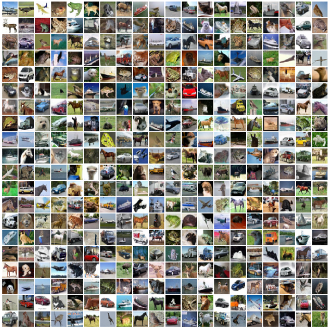
The authors present samples from CIFAR10, CelebA-HQ, and LSUN. CIFAR10 samples are highlighted in Figure 3. Comparing to the previous results in Figure 2d, it is clear that these samples are higher quality. The samples seem much crisper and clearly correspond to the classes of CIFAR10 for most images. The authors back up these observations by comparing the negative log likelihood on the CIFAR10 set to those previously reported in the original diffusion probabilistic models paper. The negative log likelihoods as wellas FID and inception scores are shown in Table 1

Ablation of Training Objectives

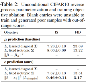
In addition to analyzing the performance of their method to prior work, the authors also investigate their design choices through an ablation experiment. In the experiment, they compare performance for models trained with fixed and learned variance schedules, along with models trained to predict the score vs those which predict the posterior mean. The results of the ablation are in Table 2.

Conclusions

In the first paper, the authors introduce Diffusion Probabilistic Models, and show experimental results on image generation. However, the the method did not generate much traction, perhaps due to the density of the notation in the original paper or the somewhat uninspiring unconditional samples on the CIFAR10 dataset. In Denoising Diffusion Probabilistic Models, Ho et al. build on the work introduced by Sohl-Dickstein et al. and by show that with some modifications, diffusion probabilistic models can produce exceptional image samples. Thanks to these two works, there has been an explosion in generative modelling methods, many of which leverage diffusion probabilistic models and denoising diffusion probabilistic models.

To Add

Put links and content here to be added. This does not need to be organized, and will not be graded as part of the page. If you find something that might be useful for a page, feel free to put it here.