Course:CPSC522/Concatenating Hyperspherical Distributions in Hyperspherical VAE

Concatenating Hyperspherical Distributions in Hyperspherical VAE

In this page, we take a look at the effects of using a concatenation of multiple independent hyperspherical distributions to extend Hyperspherical VAE proposed by Davidson et al. on single-cell RNA sequencing data.

Principal Author: Sarah Chen, Yilin Yang
Collaborators:

Abstract

As high-dimensional data becomes more and more prevalent, how to deal with high-dimensionality becomes an increasingly popular research topic. While traditionally VAEs use the Gaussian normal distribution, Davidson et al. considered using a von Mises-Fisher (vMF) distribution instead. Although they empirically showcase the power of such a distribution, they also note the limited performance in higher dimensional space. In this page, we take a look at the paper titled "Increasing Expressivity of a Hyperspherical VAE" by Davidson et al. , which claims to alleviate Hyperspherical VAE's problem with high dimensional data by considering a product-space assumption. We will first explain the improvement proposed by Davidson et al. and then empirically evaluate its performance on two high-dimensional single-cell RNA-sequencing datasets in a high dimensional latent space. In addition, we also evaluate its performance in a low dimensional latent space which the original authors did not do.

Builds on

The wiki page made by Sarah Chen: Hyperspherical Variational Auto-Encoders for the background information.

The paper we will be focusing on: Increasing Expressivity of a Hyperspherical VAE

Related Pages

Hyperspherical Variational Auto-Encoders by Davidson et al.

Introduction

Motivation

Single-cell RNA-sequencing (scRNA-seq) data is a valuable resource for inferring new biological insights such as understanding cell relationships, as well as identifying and categorizing cell types. Dimensionality reduction is a critical step for these downstream analyses. The hyperspherical variational auto-encoder, denoted as ${\mathcal {S}}$-VAE, has been demonstrated to be a powerful way of doing so. However the experiments only went up to a latent dimension of 20 and it was noted that for a 20-sphere, the ${\mathcal {S}}$-VAE became more uncertain about the embeddings. This problem could worsen as the dimension increases, but a higher dimensional latent space may be more desirable in some cases. We examine the concatenated ${\mathcal {S}}$-VAE as a potential solution to this problem.

Problem: Why do Hyperspherical VAE Suffer in Higher Dimensional Space?

As Sarah Chen's Hyperspherical Variational Auto-Encoders provides a comprehensive background on Hyperspherical VAEs, we directly introduce the problem setting.

Vanishing Surface Problem:For a hypersphere $S^{m-1}$, the surface area is described as:

$$S^{m-1}=r^{m}{\frac {2(\pi ^{m/2})}{\Gamma (m/2)}}$$

Where $m$ is dimension and $r$ is the radius, we observe that $S^{m-1}\rightarrow 0$ as $m\rightarrow \infty$, even for $m$ as small as 20, we have a very smaller surface area, and will lead to limited expressiveness in Hyperspherical VAEs in higher dimensions.

Taking a look at the vMF distribution we have:

$$q(\mathbf {z} |\mu ,\kappa )=C_{m}(\kappa )\exp {(\kappa \mu ^{T}\mathbf {z} )}$$

Where

$$C_{m}(\kappa )={\frac {\kappa ^{m/2-1}}{(2\pi )^{m/2}I_{m/2-1}(\kappa )}}$$

Here $C_{m}$ is a normalization constant. The equation for it is below. It is hard to compute and has no closed form. $I_{\nu }(.)$ is the modified Bessel function of the first kind, where $\nu$ indicates the order. Davidson et al. note that this scalar $\kappa$, also called the concentration parameter is fixed for all dimensions, thus the authors hypothesize that $\kappa$ is why Hyperspherical VAE has limited expressiveness as the dimensions are increased.

Proposed Method

Instead of using a single latent hyperspherical assumption, Davidson et al. propose to use a concatenation of multiple independent hyperspherical distributions. This composition of hyperspherical distributions effectively bypasses the concentration parameter constraint by using a $\kappa$ for each hypersphere. Therefore we can rewrite the pdf as:

$$p(\mathbf {z} )=p(\mathbf {z} _{0},\mathbf {z} _{1},\dots ,\mathbf {z} _{k}):=\prod _{i=0}^{k}p(\mathbf {z} _{i})$$

Here each hyperspherical random variable $\mathbf {z}$ is sampled from a uniform distribution naturally defined to be on a hypersphere $U(S^{m-1})$. Here we assume that each $\mathbf {z}$ is independent of the other. We will also assume the independence of the vMF posterior: ${\textstyle q(\mathbf {z} |\mathbf {x} ;\phi )=q(\mathbf {z} _{0}|\mathbf {x} ;\phi )q(\mathbf {z} _{1}|\mathbf {x} ;\phi )\dots q(\mathbf {z} _{k}|\mathbf {x} ;\phi )}$, and based on the derivations in Appendix A , we can simplify the KL divergence to:

$${KL}(q(\mathbf {z} |\mathbf {x} ;\phi )||p(\mathbf {z} ))=\sum _{i}{KL}(q(\mathbf {z} _{i}|\mathbf {x} ;\phi )||p(\mathbf {z} _{i}))$$

Degree of Freedom Trade-Off

The author of the paper notes that there is an inherent trade-off between the Degree of Freedom (dof) and the concentration parameter $\kappa$. When we only have a single hypersphere, say $S^{m+1}$, we can support up to ${m+1}$ independent feature dimensions. Therefore each dimension will have restricted flexibility as we have a single concentration parameter $\kappa$. When we use the proposed improved method, we can rewrite $S^{m+1}$ using the Cartesian cross-product $S^{m/2}\times S^{m/2}$, thus we lose an independent dimension (or dof) for increased flexibility as each hypersphere $S^{m/2}$ will have a different $\kappa$. As each concentration parameter $\kappa$ describes fewer dimensions, we result in greater flexibility.

This is in contrast to the Gaussian distribution used by standard VAEs, as the Gaussian distribution already has a concentration parameter for each dimension in the form of the covariance matrix. Therefore it does not benefit from such a formulation. In contrast, vMF only has a single concentration parameter $\kappa$ for all dimensions, using the proposed method will theoretically yield a more flexible model that should be ideal for high-dimensional data, which we aim to explore.

Hypothesis

In the following section, we will empirically evaluate the claims made by the authors by comparing the performance of the ${\mathcal {S}}$-VAE and the concatenated ${\mathcal {S}}$-VAE on two scRNA-seq datasets, which we will introduce before moving to the experiment setup. We hypothesize that the concatenated ${\mathcal {S}}$-VAE will achieve better performance than the ${\mathcal {S}}$-VAE in high dimensions and similar performance in low dimensions.

Datasets

For our two scRNA-seq datasets, we use the data provided by Cross-tissue Immune Cell Atlas, they have also linked the science article that details the datasets. Here we will briefly introduce this as most of the biological background is beyond the scope of this course.

cellxgene Matrix

A cellxgene matrix is a 2D matrix where each of the rows represents one cell and each of the columns represents a gene. The raw matrix contains counts where for a given cellxgene matrix $X$, the entry $X_{ij}$ contains the count of gene $j$ for the cell $i$.

A visualization of the myeloid cells (a) with the subgroups circled (b). The top left are the monocytes. The top right are the macrophages. Below in the center are the dendritic cells.

Myeloid Cells

Myeloid cells dataset contains a $51552\times 36601$ cellxgene matrix where 8 different cells were detected by CellTypist, a tool for automated cell type annotation by the same authors as Cross-tissue Immune Cell Atlas. After manual curation, three additional cell types were detected for a total of eleven types. Most of the individual cell types can be placed into one of three groups: macrophages, monocytes, and dendritic cells.

A visualization of the B-cells (a) with the subgroups circled (b). From left to right are the memory B-cells, the germinal center (GC) B-cells, and the plasma cells.

B-cells

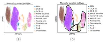
The B-cell dataset contains a $54934\times 36601$ cellxgene matrix where 6 different cells were detected by CellTypist, after manual curation, 5 additional cell types were detected for a total of eleven types. B-cells include the progenitors in the bone marrow, developmental states in lymphoid tissues, and terminally differentiated memory and plasma cell states in lymphoid and nonlymphoid tissues. Memory B-cells include ABCs which are a specific type of memory B-cells. Germinal center (GC) B-cells, both I and II, form another group and so do plasmablasts and plasma cells.

Preprocessing

Prior to running the experiments, we applied standard preprocessing steps for scRNA-seq datasets. The datasets were first normalized by the total count, scaled by 10,000, and then log-transformed. The data was further scaled to have zero mean and unit variance. As the dimensionality of the datasets was very high, highly variable genes were selected which reduce the dimensionality of each dataset to about 2000. Lastly, we account for batch effects which is variation arising from technological noise. In this case, we regress out batch effects from chemistry to remove variation between cells arising from the sequencing method used to obtain the scRNA-seq data.

Experiments

In their paper, the authors did not provide code for the proposed concatenated ${\mathcal {S}}$-VAE, therefore for the purpose of our experiments, we contacted the original authors and modified their encoder structure for our purposes as well as assumed a student-T distribution in the reconstruction term. We used three layers with 128, 64, and 32 units for the encoder and two layers with 32 and 128 units for the decoder. For the ${\mathcal {S}}$-VAE, we used an Adam optimizer with a learning rate of $1e-4$. For the concatenated ${\mathcal {S}}$-VAE, we also used an Adam optimizer but with a learning rate of $1e-5$.

We tried out dimensions of $n=2$, $n=5$, and $n=40$ for the ${\mathcal {S}}$-VAE and the concatenated ${\mathcal {S}}$-VAE. For the concatenated ${\mathcal {S}}$-VAE, we tried increasing the degrees of freedom for $n=2$ and $n=5$. For $n=40$, we tried keeping the ambient space fixed and increasing the degrees of freedom. Both balanced and unbalanced breaks were tested. The specific breakdown of subspaces for the concatenated VAE is outlined in the table below.

The ambient space, hyperspherical space, number of concentration parameters, and the product of hyperspherical spaces tested for each dataset.

After the ${\mathcal {S}}$-VAE and concatenated ${\mathcal {S}}$-VAE are trained, the datasets are fed to the models and the means of the posterior distribution $p(z\mid x)$ are output by the encoder. These means are used as low-dimensional cell embeddings for downstream analyses such as clustering.

We use k-means and k-NN to cluster and classify the cell types, and Adjusted Rand Index (ARI), Normalized Mutual Information (NMI) and Adjusted Mutual Information (AMI) for evaluation.

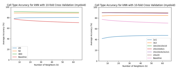
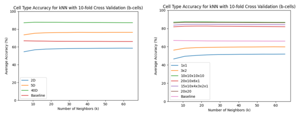
Elbow plots for k-means were used to chose the number of clusters. The x-axis is the number of clusters, and the y-axis is the distortion which is the sum of squared distances of each data point to the centroid of the cluster it is assigned to. The $k$ that is chosen is the one that causes a "kink" in the elbow. For k-NN, we split the datasets into ten folds. Nine folds were used for training and one for testing. Various $k$ were used which is shown on the x-axis, and the y-axis is the average accuracy over each of the test folds. The baseline used all of the highly variable genes kept after preprocessing of the datasets. The cell types were used as the class labels.

ARI measures the similarity between two cluster random index assignments and adjusts for chance. NMI is the Normalized version of Mutual Information between two clusterings with 0 being no mutual information and 1 for perfect correlation. AMI is the Mutual Information score that accounts for chance. It should be noted that all three evaluation metrics are invariant to the actual labels, and any permutation of class labels will not change the score.

Further details can be found in the documentation of sklearn.metrics.

Results

In the figures, the product space is denoted as $d_{1}\times d_{2}\times ...\times d_{m}$ where $d_{i}$ is the dimension of the $ith$ subspace and there are $m$ subspaces. For example, $[{\mathcal {S}}_{1}]_{\times 2}$ would be $1\times 1$. Clusterings are shown for the product space with the best performance and the product space with the worst performance. Performance was measured by the clustering metrics with better-performing product spaces having scores closer to 1.

Myeloid Cells

Inferring the number of cell types

Regardless of the dimension $n$ when using the ${\mathcal {S}}$-VAE, basing the number of cell types on where a "kink" in the elbow appeared would result in the number being underestimated. The "kink" typically appeared around $k=4$ to $k=6$ while the true number of types was 11.

Elbow plots for the ${\mathcal {S}}$-VAE from left to right for $n=2$, $5$, and $40$.

For the concatenated ${\mathcal {S}}$-VAE, the number of cell types was also underestimated. For $n=40$, the underestimation got worse as the "kink" consistently appeared around $k=3$ to $k=4$ although the "kink" was smoother for $[{\mathcal {S}}_{20}]_{\times 2}$.

Elbow plots for the concatenated ${\mathcal {S}}$-VAE from left to right for $[{\mathcal {S}}_{1}]_{\times 2}$, ${\mathcal {S}}_{3}\times {\mathcal {S}}_{2}$, ${\mathcal {S}}_{15}\times {\mathcal {S}}_{10}\times {\mathcal {S}}_{4}\times {\mathcal {S}}_{3}\times {\mathcal {S}}_{2}\times {\mathcal {S}}_{1}$, and $[{\mathcal {S}}_{20}]_{\times 2}$.

k-means Clustering

${\mathcal {S}}$-VAE

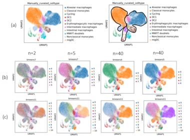
When comparing the clusterings with $k$ chosen from the elbow plot, the results were similar. The monocytes and macrophages tended to get grouped together whereas the dendritic cells and doublets were more mixed with one another. With $n=5$ though, there was a noticeable improvement when using clustering with $k=11$ as some of the nonclassical monocytes began to form a separate cluster from the classical monocytes and the doublets formed their own cluster. It was a similar case for $n=40$ with $k=11$.

The true cell types for the ${\mathcal {S}}$-VAE with subgroups circled in black on the right (a). The clustering results for choosing $k$ with the elbow plot (b) and $k=11$ (c), from left to right, for $n=2$, $5$, and $40$.

Concatenated ${\mathcal {S}}$-VAE

While the ${\mathcal {S}}$-VAE with $n=2$ had a decent performance, the concatenated one performed very poorly as the cell types were all mixed together in the clusters. For $n=5$, the monocytes were split more distinctly between classical and non-classical but it was not entirely correct as some classical monocytes were being included with the nonclassical ones. For $n=40$, performance was similar to using the non-concatenated ${\mathcal {S}}$-VAE. Shown in the below figure are the clusterings for the worst (${\mathcal {S}}_{15}\times {\mathcal {S}}_{10}\times {\mathcal {S}}_{4}\times {\mathcal {S}}_{3}\times {\mathcal {S}}_{2}\times {\mathcal {S}}_{1}$) and best ($[{\mathcal {S}}_{20}]_{\times 2}$) product space with $n=40$. There was not much of a difference except with the intermediate macrophages. When $n=40$, the ARI, AMI, and NMI scores were 0.69, 0.61, and 0.61 for the worst performing product space and for the best performing product space, the ARI, AMI, and NMI scores were 0.75, 0.66, and 0.66 for the clusterings where $k$ was chosen from the elbow plot. In all cases, the concatenated ${\mathcal {S}}$-VAE failed to distinguish between the dendritic cells.

The true cell types for the ${\mathcal {S}}$-VAE with subgroups circled in black on the right (a). The clustering results for choosing $k$ with the elbow plot (b) and $k=11$ (c), from left to right, for $[{\mathcal {S}}_{1}]_{\times 2}$, ${\mathcal {S}}_{3}\times {\mathcal {S}}_{2}$, ${\mathcal {S}}_{15}\times {\mathcal {S}}_{10}\times {\mathcal {S}}_{4}\times {\mathcal {S}}_{3}\times {\mathcal {S}}_{2}\times {\mathcal {S}}_{1}$, and $[{\mathcal {S}}_{20}]_{\times 2}$.

k-NN Classification

The ${\mathcal {S}}$-VAE worked better for the lower dimensions particularly for $n=2$ as the accuracy was much higher. The performance between the ${\mathcal {S}}$-VAE and concatenated ${\mathcal {S}}$-VAE, regardless of the product space used, was similar for $n=40$. These results agree with the performance of the clusterings.

Average accuracy of myeloid cell type classification using k-NN with 10-fold cross validation for the ${\mathcal {S}}$-VAE and the concatenated ${\mathcal {S}}$-VAE.

B-cells

Inferring the Number of Cell Types

For the ${\mathcal {S}}$-VAE, using an elbow plot to choose the number of clusters for the B-cells would also cause the number of cell types to be underestimated. The true number was 11 but the "kink" appeared around $k=6$ to $k=7$.

Elbow plots for the ${\mathcal {S}}$-VAE from left to right, for $n=2$, $5$, and $40$.

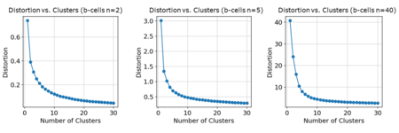
Using the concatenated ${\mathcal {S}}$-VAE, the results were similar to using the ${\mathcal {S}}$-VAE. Like the myeloid cells, the number of breaks or whether the breaks were balanced or unbalanced did not affect the elbow plot for $n=40$.

Elbow plots for the concatenated ${\mathcal {S}}$-VAE from left to right for $[{\mathcal {S}}_{1}]_{\times 2}$, ${\mathcal {S}}_{3}\times {\mathcal {S}}_{2}$, ${\mathcal {S}}_{20}\times {\mathcal {S}}_{10}\times {\mathcal {S}}_{6}\times {\mathcal {S}}_{1}$, and $[{\mathcal {S}}_{20}]_{\times 2}$.

k-Means Clustering

${\mathcal {S}}$-VAE

Unlike the myeloid cells, the clusterings across all dimensions were poor. It was especially bad for $n=2$ since the cells were all essentially mixed no matter the type. Performance improved slightly for $n=5$ and $n=40$ with $n=5$ seeming better since the plasma cells formed their own cluster. However, no matter the dimension, clusters tended to be split into two large groups without much granularity since types with few cells, such as doublets and ABCs, would get clustered with other cells.

The true cell types for the ${\mathcal {S}}$-VAE with subgroups circled in black on the right (a). The clustering results for choosing $k$ with the elbow plot (b) and $k=11$ (c), from left to right, for $n=2$, $5$, and $40$.

Concatenated ${\mathcal {S}}$-VAE

The concatenated ${\mathcal {S}}$-VAE failed to properly cluster the cell types for $n=2$ and $n=5$ whether $k$ was set using the elbow plot or set to $11$. The one exception for the plasmablasts for $n=5$ and $k=11$. The ${\mathcal {S}}$-VAE had better performance overall for $n=5$ though. When $n=40$, the ARI, AMI, and NMI scores were 0.15, 0.27, and 0.27 for the worst performing product space and for the best performing product space, the ARI, AMI, and NMI scores were 0.30, 0.39, and 0.39 for the angles where $k$ was chosen from the elbow plot. For $n=40$ and $k=11$, using ${\mathcal {S}}_{20}\times {\mathcal {S}}_{10}\times {\mathcal {S}}_{6}\times {\mathcal {S}}_{1}$ helped separate the three rightmost cell types: T/B doublets, plasmablasts, and plasma cells. In contrast, for $n=40$ and $k=5$, using $[{\mathcal {S}}_{20}]_{\times 2}$ improved the separation of the naive B-cells and memory B-cells. This seemed like a slight improvement over just the ${\mathcal {S}}$-VAE, but the clusterings still had some other cells mixed in though and smaller clusters were not detected.

The true cell types for the ${\mathcal {S}}$-VAE with subgroups circled in black on the right (a). The clustering results for choosing $k$ with the elbow plot (b) and $k=11$ (c), from left to right, for $[{\mathcal {S}}_{1}]_{\times 2}$, ${\mathcal {S}}_{3}\times {\mathcal {S}}_{2}$, ${\mathcal {S}}_{20}\times {\mathcal {S}}_{10}\times {\mathcal {S}}_{6}\times {\mathcal {S}}_{1}$, and $[{\mathcal {S}}_{20}]_{\times 2}$.

k-NN Classification Accuracy

Notably, the concatenated ${\mathcal {S}}$-VAE performed worse for the low dimensions. For $n=40$, the product space did affect the accuracies. Uneven breaks had lower accuracies while even breaks achieved similar results to the un-concatenated ${\mathcal {S}}$-VAE. There also seemed to be a small preference for a higher number of breaks as ${\mathcal {S}}_{15}\times {\mathcal {S}}_{10}\times {\mathcal {S}}_{4}\times {\mathcal {S}}_{3}\times {\mathcal {S}}_{2}\times {\mathcal {S}}_{1}$ (purple) is above ${\mathcal {S}}_{20}\times {\mathcal {S}}_{10}\times {\mathcal {S}}_{6}\times {\mathcal {S}}_{1}$ (red) and $[{\mathcal {S}}_{10}]_{\times 2}$ (green) is very slightly above $[{\mathcal {S}}_{20}]_{\times 2}$ (brown).

Average accuracy of B-cell type classification using k-NN with 10-fold cross validation for the ${\mathcal {S}}$-VAE and the concatenated ${\mathcal {S}}$-VAE.

Discussion

Performance in High Dimensions

The concatenated ${\mathcal {S}}$-VAE achieved only a similar performance to the ${\mathcal {S}}$-VAE. Noting that results of the ${\mathcal {S}}$-VAE at $n=40$ were not much different than at $n=5$, it may be the case that the concatenated ${\mathcal {S}}$-VAE will show its benefits most when the dimension of the latent space starts to become so high that it negatively impacts the performance of the ${\mathcal {S}}$-VAE.

Running the concatenated ${\mathcal {S}}$-VAE for more epochs may also eventually result in it achieving better performance than the ${\mathcal {S}}$-VAE since the concatenated ${\mathcal {S}}$-VAE was only run for 10 epochs. The ${\mathcal {S}}$-VAE was run for about 3 epochs. In contrast, the models in scPhere were run for 500 epochs for a dataset of this size. The reason we used a low number of epochs was that we would encounter NaN values past that. This was after decreasing the learning rate, which partially helped, as the issue was worse when it was higher. Additionally, more hyperparameter tuning may be beneficial. For example, we used the same default architecture as scPhere so it may be worth trying deeper networks and adjusting the number of units per layer.

Regarding how the space should be broken up and the number of subspaces, we found a slight preference for balanced breaks. The authors mention that this is because if the breaks are uneven, the model could end up ignoring some subspace channels which is problematic if it ignores higher-dimensional subspaces in favour of lower ones. No preference could be seen for the number of breaks which may be because since the minimum and maximum number was 2 and 6, the difference was not significant enough to have much of an impact.

Performance in Low Dimensions

For lower-dimensional parts, we followed the analysis conducted by Davidson et al. and tried both models on MNIST with $n=5$. The concatenated ${\mathcal {S}}$-VAE performed slightly worse by all metrics, which might indicate that it’s not suitable for lower dimensions. As for intuition behind this result, we think it may come from tuning or the dof trade-off, Although it could be that we may have chosen a poor set of hyperparameters, we think it's likely due to flexibility trade-off being adverse to our concatenated ${\mathcal {S}}$-VAE model, as we likely won't need more concentration parameters for such a low dimensional task.

Performance on the Myeloid Dataset vs. the B-cells Dataset

Using the embeddings from both models resulted in clusterings of the major groups with $k$ chosen from the elbow plot. The granularity of the cell types was more variable. Specifically, performance was consistently better for the myeloid dataset than the B-cells dataset. This may be because cell types within a subcategory for the myeloid dataset are more distinguishable from one another and are illustrated by the intermediate macrophages tending to be separated from the alveolar macrophages. For the B-cells, they may be more similar, such as the memory B-cells and ABCs or plasma cells and plasmablasts. There was a similar problem with the monocytes in the myeloid dataset. The cell types of the B-cells dataset are also determined by the maturity level of the B-cell until it eventually differentiates into a memory B-cell or plasma cell. Plasma cells may be more clearly distinguishable whereas the rest are more similar since they are essentially the same cell but at different points in time. As a more complicated dataset, the number of epochs then may be too low for the B-cells as mentioned in in Performance in High Dimensions. The good performance of the ${\mathcal {S}}$-VAE though on the myeloid dataset further suggests the appropriateness of the ${\mathcal {S}}$-VAE for scRNA-seq data.

Conclusion

Overall, the experiments do not support our hypothesis. The ${\mathcal {S}}$-VAE performed better than the concatenated ${\mathcal {S}}$-VAE in low dimensions and the concatenated ${\mathcal {S}}$-VAE did not demonstrate an improvement in performance for $n=40$. It may be the case that steps as discussed could be taken to resolve this, but when using a high latent dimension, it seems difficult to say for certain whether the issue lies with the concatenated ${\mathcal {S}}$-VAE itself or hyperparameter tuning without further experimentation. In the meanwhile, it seems more appropriate to use the ${\mathcal {S}}$-VAE for scRNA-seq data.