Neural Architecture Search

Title

Neural Architecture Search

Principal Author:
Anubhav Garg

Abstract

The challenge of Neural Architecture Search (NAS) is addressed by two papers, DARTS and ProxylessNAS, which are compared in this article. DARTS has succeeded in substantially decreasing the computation time required for NAS, from several hundred GPU hours to just a few hours. ProxylessNAS, on the other hand, has overcome the memory explosion problem experienced by DARTS by using path binarization and starting from a backbone network to derive the final network architecture. These methods signify significant advancements in NAS, and when choosing an approach for a particular task, it is important to consider the strengths and limitations of each.

Builds on

This page builds on these two papers -

1. DARTS : https://arxiv.org/abs/1806.09055 2. ProxylessNAS : https://arxiv.org/pdf/1812.00332.pdf

Related Pages

Course:CPSC522/Reinforcement Learning was used initially to solve the problem of NAS. Apart from this evolutionary algorithms were also used before.

Content

Automatic Machine Learning or AutoML in short are a set of methods to automate the machine learning process to a certain extent, which can be as simple as tuning the hyperparameters of a machine learning model to automatically coming up with a neural network architecture. The former is referred to as hyperparameter tuning, and the latter is called Neural Architecture Search (NAS). In this article I will be discussing two NAS papers, namely DARTS and ProxylessNAS.

To give a background about DARTS, basically before it NAS was very compute intensive, since it required to evaluate many different architectures possible for a given task and dataset. DARTS made this discrete problem scalable by adding a continuous parameter to the architecture. Before DARTS, reinforcement learning and evolution based models were popular for NAS.

1.DARTS

Prelims

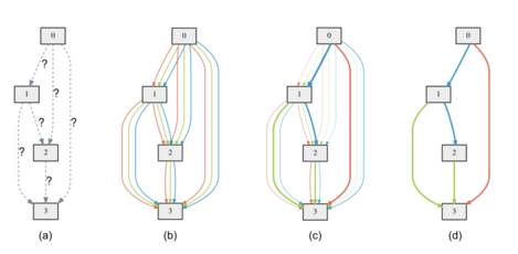
A cell refers to an ordered sequence of N nodes represented by a directed acyclic graph. In this cell, each node (i) denotes a latent representation that could act as a feature map in convolutional networks. Additionally, every directed edge (i, j) present in the cell is linked to an operation o (i,j), which transforms the node x (i). The cell comprises two input nodes and a single output node. In convolutional cells, the output nodes of the cell are defined as the ones in the previous two layers. However, in recurrent cells, the input nodes are identified as the current step input and the state that has been carried from the previous step. To obtain the cell's output, a reduction operation such as concatenation is applied to all intermediate nodes. Each preceding node plays a part in the calculation of all intermediate nodes: $x_{j}=\sum \limits _{i=1}^{j-1}o_{i,j}x_{i}$

(a) The operations on the edges are not known initially. (b) The search space is gradually expanded by placing a variety of potential operations on each edge. (c) The mixing probabilities and network weights are optimized together through solving a bilevel optimization problem. (d) The final architecture is derived from the optimized mixing probabilities.

Method

The collection of possible operations is denoted as O, which includes convolution, max pooling, or zero. Each operation is represented by an o(·) function that acts on x(i). To create a continuous search space, the categorical selection of an operation is replaced with a softmax function over all possible operations: ${\bar {o}}{i,j}(x)={\frac {\sum \limits {o\in O}e^{\alpha _{i,j,o}}\cdot o(x)}{\sum \limits _{o'\in O}e^{\alpha _{i,j,o'}}}}$ The weights that combine the operations for a node pair (i, j) are represented by a vector alpha(i,j) of size |O|. By jointly learning a set of continuous variables alpha = {alpha(i,j)} and the weights w for all mixed operations (e.g., convolution filter weights), a discrete architecture can be found by substituting each mixed operation o-bar(i,j) with the operation that is most likely: $o_{i,j}=\arg \max \limits _{o\in O}\alpha _{i,j,o}$ Alpha is referred to as the architecture encoding. After relaxation, the goal is to minimize the validation loss $L_{val}(w^{,}\alpha ^{)}$ using gradient descent, where both the training loss Ltrain and validation loss Lval depend on the architecture alpha and the weights w in the network. The objective is to find alpha* that minimizes $L_{val}(w^{,}\alpha ^{)}$, where the weights w* associated with the architecture are obtained by minimizing the training loss $w^{*}=\operatorname {argmin} _{w}L_{\operatorname {train} }(w,\alpha ^{*})$. This creates a bilevel optimization problem, where alpha is the upper-level variable and w is the lower-level variable, using the approach of architecture search via RL or evolution.

To make each node in the discrete architecture, the algorithm picks the strongest operations (from different nodes) among all non-zero options from the previous nodes. To keep things consistent with previous studies, the algorithm sets k to 2 for some types of nodes and 1 for others. Zero operations are not included for two reasons. Firstly, the algorithm needs a certain number of incoming edges per node that are not zero to compare fairly with other models. Secondly, the strength of zero operations is not clear because changing the logits of zero operations only changes the size of the resulting node representations, and does not change the final classification result due to batch normalization.

Results

Here I present the results of the architectures found by DARTS -

The following table shows a comparison between various image classifiers on CIFAR-10 dataset, where lower error rate indicates better performance. It is important to note that the search cost for DARTS does not take into account the selection cost of 1 GPU day, or the final evaluation cost of training the chosen architecture from scratch, which takes 1.5 GPU days.

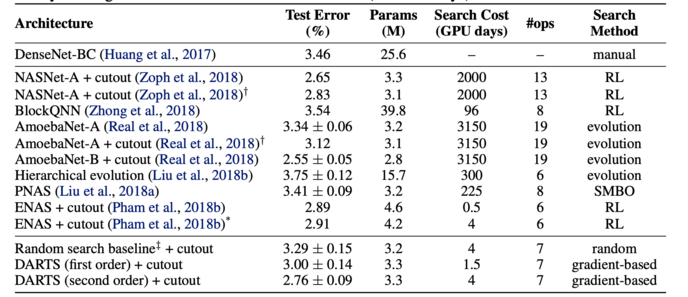
On Table 1, the convolutional architectures' results on CIFAR-10 are displayed. Notably, DARTS attained similar outcomes as the current state-of-the-art methods while utilizing far fewer computational resources (1.5 or 4 GPU days compared to 2000 GPU days for NASNet and 3150 GPU days for AmoebaNet). Furthermore, DARTS outperformed ENAS by discovering cells with similar error rates but fewer parameters, although the search time was slightly longer due to the repeated search process four times for cell selection. However, this is less critical for convolutional cells because the discovered architectures' performance is not highly reliant on the initialization.

Comparison of DARTS with state-of-the-art language models on PTB. Lower perplexity values are better. However, it's important to note that the search cost for DARTS doesn't include the selection cost, which takes 1 GPU day, or the final evaluation cost, which requires training the chosen architecture from scratch and takes 3 GPU days.

Comparison of mobile image classifiers with state-of-the-art models on ImageNet.

The last table gives the result of the architecture searched on CIFAR-10 and evaluated on Imagenet.

2. ProxylessNAS

As seen above, DARTS was able to reduce the computation time by order of magnitude in comparison to prior approaches. However, the whole one-shot architecture ((b) in first figure of DARTS) needed to be kept in memory, which depends on the number of operations in the search space.

This paper tried to solve this problem with an added advantage of searching directly on the dataset of choice.

Prelims

They search on an-overparametrized network also called the parent network. This parent network can be represented as a directed acyclic graph (DAG) denoted as $G=(V,E)$ , where nodes $v\in V$ represent intermediate representations and edges $e\in E$ represent various transformations of those representations such as pooling and convolution. Multiple edges $e_{ij}$ exist between every pair of nodes $v_{i}$ and $v_{j}$ to cover all possible architectures within the search space. A NAS algorithm is used to train architecture parameters, which are represented by the weight $\alpha$. The architecture weight with the highest value is chosen for every node pair to obtain the final network known as the child network.

Method

In order to retrieve the output feature maps of all N paths, they are computed and subsequently saved in the memory. Nevertheless, training a compact model necessitates only a solitary path. This implies that executing the One-Shot and DARTS techniques consume roughly N times the amount of GPU memory and GPU hours needed to train a compact model. This can pose difficulties when working with vast datasets since it can readily go beyond the memory limits of hardware that has a large design space.

To minimize memory requirements, a solitary path is exclusively maintained while training the over-parameterized network. They use the approach in which entire paths are binarized. This involves introducing a set of N real-valued architecture parameters denoted by $\alpha$ and then transforming the real-valued path weights to binary gates:

By using binary gates instead of real-valued path weights (as done to DARTS) and illustrated in Eq. (3), it is ensured that only one active path of activation exists in memory at run-time. This decrease in memory requirements during the training of the over-parameterized network is equivalent to the memory requirements of training a compact model, leading to more than ten times memory savings.

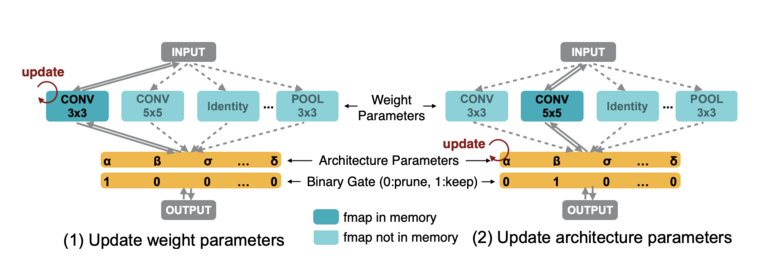
The process of training the weight parameters and binarized architecture parameters in the over-parameterized network is shown in the above figure. Initially, the architecture parameters are frozen, and for each batch of input data, binary gates are randomly sampled using Eq. (2) to train the weight parameters. Then, the weight parameters of active paths are updated using standard gradient descent on the training set (left). In contrast, when training the architecture parameters, the weight parameters are held constant, and the architecture parameters are reset. The architecture parameters are then updated on the validation set (right). These two update steps are performed alternatively. Once the training of architecture parameters is complete, the redundant paths are removed to derive the compact architecture. The path with the highest path weight is selected in this study. Unlike weight parameters, architecture parameters are not directly involved in the computation graph and therefore cannot be updated using standard gradient descent.

In the process of updating architecture parameters, two paths are chosen randomly based on the multinomial distribution (p1, · · · , pN). The remaining paths are then masked, temporarily reducing the candidate pool from N to 2. The weights {pi} and binary gates {gi} of the masked paths are reset accordingly. Using gradients calculated, the architecture parameters of the two selected paths are updated. The values of the updated architecture parameters are rescaled by multiplying a ratio to ensure that the weights of unselected paths remain unchanged. This causes one of the selected paths to have increased weight and the other to have decreased weight, while all other paths remain unaltered. This method ensures that memory requirements are reduced to the level of training a compact model, as only two paths are involved in each architecture parameter update step, regardless of the value of N.

Results

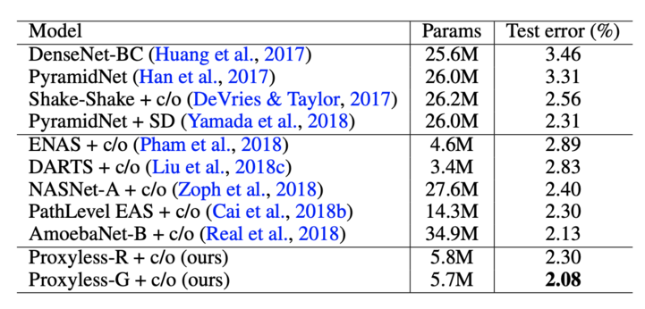
In below table, a summary of test error rate outcomes for the proposed method and other contemporary frameworks on CIFAR10 is presented. "c/o" denotes the implementation of Cutout.

The proposed method outperforms current architectures by achieving a reduced test error rate and better parameter efficiency. For instance, Proxyless-G achieves a test error rate of 2.08%, slightly better than AmoebaNet-B's previous optimal architecture on CIFAR-10. Notably, the proposed model uses only 5.7M parameters, which is a six-fold reduction from AmoebaNet-B's 34.9M parameters. Additionally, Proxyless-G and Proxyless-R (variation to default) achieve equivalent or better test error rate outcomes with only half the number of parameters compared to PathLevel EAS, which also explores the tree-structured architecture space. The empirical results of the proposed ProxylessNAS demonstrate the advantages of directly exploring a broad architecture space instead of repetitively stacking the same block.

cifar10

Similarly, the below figures displays results for ImageNet dataset with latency measures.

Imagenet

Conclusions

In this article, I compared two papers, DARTS and ProxylessNAS which solves the problem of Neural Architecture Search. We saw that how DARTS reduced the computation time of NAS from 100s of GPU hours to a few hours. ProxylessNAS reduced the memory explosion of DARTS by starting from a backbone network and using path binarization to derive the final network.