Course:CPSC532:StaRAI2020:Variance Reduction and Convergence Analysis in BBVI

Title

Variance Reduction and Convergence Analysis in BBVI

Authors: Mohamad Amin Mohamadi

Abstract

This page evaluates three hypotheses about the blackbox variational inference algorithm. The hypotheses are listed as follows:

1. Rao-Blackwellization and Control Variates can decrease the variance of the estimated gradients used in converging towards the optimal latent variables for the proposals.
2. These reductions in the variance of the estimated gradients help the algorithm converge significantly faster.
3. Blackbox variational inference methods can perform inference over the given models faster than traditional sampling methods if used in conjunction with variance reduction techniques.

Related Pages

You can find more information about variational inference and the blackbox variational inference algorithm here.

Content

Introduction

Variational inference is one of the widely used method to approximate posteriors in complex latent variables models. However, as deriving a variational inference algorithm generally requires some model-specific information regarding the problem and analysis, practitioners have started to formulate the variational inference problem as an optimization problem instead of trying to analytically solving it and derive the gradients based on the estimated lower bound of the variational inference objective function. This way, the algorithm can be applied to new models with little effort and without requiring the user to analytically derive model-specific closed-form solutions. Through the optimization-based approach, practitioners calculate the noisy gradients from Monte Carlo samples that are derived from the original variational distribution. Note that because we're using Monte Carlo sampling methods, no model-specific computation is required. Thereafter, through the stochastic optimization of the variational objective using the derived gradients, they infer the optimal latent variables for the proposals.

Although this approach seems promising, the variance of the estimated gradients in Monte Carlo estimations seems to introduce problems in this algorithm. The authors of the original blackbox variational inference paper have proposed a couple of methods based on Rao-Blackwellization and Control Variates to reduce the variance of the gradient, which they claim to be solving this issue. In this page, we try to implement the proposed algorithm with the suggested methods to reduce the variance of the gradient, and test them on a couple of methods to validate the claim.

Hypotheses

We first start with a validation check of the variance of the estimated noisy gradients based on the MC samples. Specifically, we hypothesize that using the Control Variates after deriving the noisy gradient estimates, the variance of the estimations must be significantly lower than the raw gradients after applying the Control Variates method. Note that we should also be concerned about the convergence of the full model because the suggested method should also keep the estimations unbiased. However, as long as they both converge, we do not care about the convergence rate here.

Second, we focus on the convergence rates, rather than the variance of the estimations for the noisy gradient. To be more specific, we hypothesize that using Control Variates method on the estimated gradients helps the algorithm have a higher convergence rate in terms of the KL divergence against the posterior. Note that unlike in the first hypothesis, we do not care about the variance of the estimations here.

Third, we would like to compare the performance of these algorithms against the traditional MCMC sampling algorithms to derive the posterior. The hypothesis here is that the blackbox variational inference algorithm provides better inference results from the posterior rather than the traditional importance sampling algorithm. To evaluate this, we can compare the parameters of the inferred posteriors using these two approaches or compare the KL Divergence of the proposals against the true posterior.

Method

In order to test and evaluate our hypotheses, we should first haven an implementation of:

• Blackbox variational inference algorithm
• A couple of well-known distributions to use as proposals with methods to calculate likelihoods of draws from them
• Differentiation calculation of mainstream distributions (to calculate the noisy gradient estimates)
• A stochastic optimization algorithm to optimize the latent variables
• KL Divergence between the true posteriors and the optimized proposals
• A framework for calculating the posterior of a model using Importance Sampling MCMC method.

We use the PyTorch framework in our implementation. The PyTorch framework has the implementations of the distributions that we need, the KL Divergence calculation and most importantly, the PyTorch's AutoGrad framework which helps us with the automatic differentiation of the objective functions that we need. As we already know, in BBVI, our goal is to learn a (factorized) approximation to posterior by maximizing the evidence lower bound through this formula:

$${\begin{aligned}{\mathcal {L}}(\lambda )&:=\mathbb {E} _{q(X;\lambda )}[log{\frac {p(Y,X)}{q(X;\lambda )}}]\\&=logp(Y)-D_{KL}(q(X;\lambda )\;||\;p(Y,X))\leq logp(Y)\\\end{aligned}}$$

Through the calculation of this estimation of the noisy gradient:

$${\begin{aligned}\nabla _{\lambda }{\mathcal {L}}(\lambda )&:=\sum _{l=1}^{L}\nabla _{\lambda }\log q(X^{l};\lambda )(\log W^{l}-{\hat {b}})\\\end{aligned}}$$

where $X^{l}\sim q(X;\lambda )$ and $W^{l}=p(Y^{l},X^{l})/q(X^{l};\lambda )$ and ${\hat {b}}$ is the variance reduction term.

For calculating the variance reduction term ${\hat {b}}$, we are going to use the Control Variates approach. According to this approach, we can rewrite a function $f(z)$ as:

$${\hat {f}}(z)\triangleq f(z)-a\left(h(z)-E[h(z)]\right)$$

Thus, ${\hat {f}}(z)$ is an unbiased estimator of $f(z)$. This way, we can control the variance of $f(z)$ through carefully defining the $h(z)$ function. Detailed explanation of the choice for $h(z)$ is available in the original paper's section 3.2 and we're not going to repeat them here. In short, we just need the calculation of some extra parameters based on the retrieved gradients from PyTorch's AutoGrad framework to apply the variance reduction term to the gradient estimates and implement the algorithm. In order to use the naive version, we just have to set ${\hat {b}}$ to zero to avoid using the variance reduction.

Moreover, there are a lot of Importance Sampling inference libraries available in python which we can use to have an implementation of the mentioned algorithm and compare its output against our implementation of BBVI.

Experiments

Experiment 1: Simple Gaussian Unknown Mean PGM

Figure 1: Gaussian Unknown Mean Model

For this experiment, we use a simple model and try to retrieve the estimation of one of the latent variables of the model. The probabilistic graphical model for this experiment is visualized in Figure 1. According to this model, we have the observation of 7 and 8, for the Model ${\mathcal {N}}\left({\mathcal {N}}(\mu _{1}=1,\sigma _{1}={\sqrt {5}}),\sigma _{2}={\sqrt {2}}\right)$ and we want to retrieve the posterior for $\mu _{1}$.

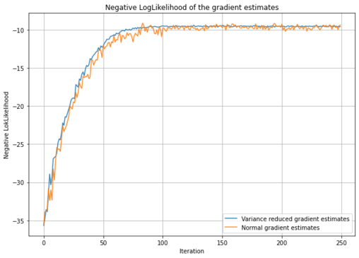
We performed inference on this model using the BBVI algorithm with Control Variates and without Control Variates. As shown in Figure 2, the Control Variates certainly have influenced the variance of the noisy gradient's estimates.

Figure 2: Negative LogLikelihood of The Gradient Estimates for the Gaussian Unknown mean model

We have listed the estimations of mean and variance for the parameter $\mu$ based on the mentioned algorithms in the following table. According to this experiment, the Control Variates slightly reduce the variance of the noisy gradient estimates, which result in slightly better convergence, but the difference is not significant. This might be due to the model being so small which results in easy computations of noisy gradient, even without variance reduction. For the next experiment, we move onto a more complex case.

Table 1: Convergence Comparison for Gaussian Unknown Mean Experiment

Statistic	True Value	Values Estimated Using BBVI	Values Estimated Using BBVI + Control Variates
Mean	7.25	7.38	7.24
Standard Deviation	0.91	0.71	0.82

Experiment 2: Bayesian Linear Regression

Figure 3: Bayesian Linear Regression Graphical Model

For this experiment, we use a bayesian linear regression model and try to retrieve the estimation of two of the latent variables of the model. The probabilistic graphical model for this experiment is visualized in Figure 3. In this task, we observe a couple of $y_{i}$ values. Give a prior over the input $x_{i}$ variables, which in this case would be a ${\mathcal {N}}(0,10)$ for each. We observe the value of $y_{i}={\text{sample from }}{\mathcal {N}}(slope\,*\,x_{i}+bias)$. The values for $X$ vector in our experiment were $[1.,2.,3.,4.,5.,6.]$ and for $Y$ we used $[2.1,3.9,5.3,7.7,10.2,12.9]$. The experiment is a well known experiment for inference on bayesian linear regression. The true values for $bias$ and $slope$ are $2.15$ and $-0.5$.

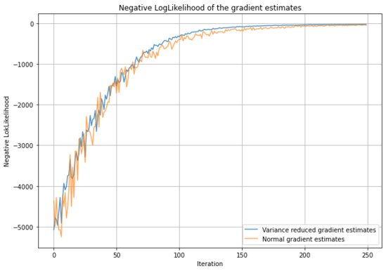
Again, we performed inference on this model using the BBVI algorithm with Control Variates and without Control Variates. As shown in Figure 4, the Control Variates certainly have influenced the variance of the noisy gradient's estimates.

Figure 4: Negative LogLikelihood for Bayesian Linear Regression

This time, the reduction in the variance of the noisy gradient estimates seems way more significant. We have listed the estimations of mean of the parameters $slope$ and $bias$ based on the mentioned algorithms in the following table. According to this experiment, the Control Variates significantly reduce the variance of the noisy gradient estimates, which result in better convergence, but the difference is not significant.

Table 2: Convergence Comparison for Bayesian Linear Regression Experiment

Statistic	True Value	Values Estimated Using BBVI	Values Estimated Using BBVI + Control Variates
Mean of $slope$	2.15	2.26	2.16
Mean of $bias$	-0.5	-0.96	-0.60

Experiment 3: Hidden Markov Model

HMM model

For this experiment, we use a hidden markov model and try to retrieve the estimation of all of the hidden latent variables of the model. The probabilistic graphical model for this experiment is visualized in Figure 4. In this task, we observe a couple of $x_{i}$ values. Give a prior over the input $z_{i}$ variables, which in this case would be a categorical distribution for each. We observe the value of $x_{i}$ based on a Gaussian distribution with mean $z_{i}$ and variance of 1, where each of these $z_{i}$s can make a transition to another $z_{j}$ based on a categorical distribution. We perform inference over all $x_{i}$s.

Once more, we performed inference on this model using the BBVI algorithm with Control Variates and without Control Variates. This time, surprisingly, as shown in Figure 5, the algorithm does not seem to converge. This is probably due to the large number of hidden variables of the model and the resulting small log likelihood weight that is the product of weights of all latent variables because of the mean field assumption. Although none of these methods converge, it seems like the variance reduction terms are helping the model have some enhancements over the estimates, whereas the normal model does not seem to work at all.

Figure 5: Negative LogLikelihood for Hidden Markov Model

Figure 6. Results of applying Metropolis-Hastings sampling algorithm on Hidden Markov Model

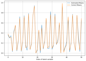
In order to check the feasibility of conducting inference over this problem, we used $pymc$'s "Metropolis Hastings MCMC" sampling approach to infer the posterior. The results for this experiment are shown in Figure 6. As shown in the figure, the MH algorithm infers the means of the Gaussian posteriors pretty accurately and outperforms the BBVI algorithm. This is, as mentioned, mainly due to the large number of latent variables in this model and the mean field assumption which is most likely not correct. A weakness of BBVI algorithm here is that if we don't make the mean field assumption, we can not implement the algorithm without requiring model-specific analytical derivations of the posterior and if do make that assumption, we're left with infinitely small likelihoods.

Conclusion

We implemented the BBVI algorithm with Control Variates on PyTorch. We hypothesized three different hypotheses regarding this algorithm. We designed three experiments with the complexity levels of small, medium and hard in terms of conducting inference over the used model's latent variables. We ran the BBVI algorithm with and without Control Variates and measured the noisy gradient estimates' negative log likelihood variance to check our hypotheses. We compared the results of the inferences with the true values of the posteriors. We used $pymc$'s implementation of Metropolis-Hastings sampling method to infer the posterior estimates and compare them with the result from BBVI. Finally, based on the experiments conducted, we conclude that:

• First hypothesis is confirmed. According to the experiments, the Control Variates in BBVI significantly reduce the variance of the estimations for noisy gradients.
• Second hypothesis is confirmed. According to the experiments, the reduction in the variance of the estimations of the noisy gradients leads to faster and more stable convergence of the proposals to the posteriors in BBVI, and also enhance the accuracy of the estimations.
• Third hypothesis is rejected. Based on the last experiment, it seems like even with Control Variates variance reduction term, the BBVI algorithm fails to converge when the model size passes a certain threshold and we must rely on the good-old MCMC sampling approaches to infer the posterior. However, they are extremely slower than the BBVI method.

For future work, we would suggest investigating the reason of the small log likelihoods for the BBVI algorithm in large models, and trying to find another Control Variate of the ELBO's gradient estimates that has more likelihood and can result in better posterior inference in large models.