Course:CPSC522/Treatment of Missing Data

Title: Treatment of Missing Data

This page introduces the problem of missingness, the three main categories of missingness, and common methods used to treat missing data in doing inference and machine learning.

Principal Author: Nam Hee Gordon Kim

Abstract

Sensors are often noisy and unreliable. We observe missingness in data, which is a phenomenon where one ore more entries of data collected from the same population is missing due to some hindrance or loss. In this page, we introduce the three fundamental categories of assumptions regarding missingness: MCAR (missing completely at random), MAR (missing at random), and NMAR (not missing at random). We formalize these definitions and introduce methods for treating missingness (or the lack thereof) when each assumption is made for inference. We introduce the imputation method which generates the "best guess" for the missing entries by reasoning on the available observed data and show the limitations of imputation.

Builds on

• Probability
• Graphical Models
• Machine Learning: Supervised, Unsupervised, Semi-Supervised

Content

Motivation

Data collection mechanisms are inherently noisy, and therefore it is difficult to guarantee the completeness of data. For example, a person taking a survey may omit one of the responses either by mistake or intentionally, and surveyors usually do not have much control over whether he/she does so. For another example, a DNA sequencer may aim to sequence the whole genome of an organism, but only a subset of the genome may end up being sequenced. In these cases, probabilistic models and methods must conduct inference with missingness in order to perform as best as they can given the missing data.

Depending on the assumption about the manner in which the data are missing, the treatment of missing data can cause wildly different results. For example, in cases where data are missing purely by chance (or missing completely at random; MCAR), simply removing the examples and/or features with missing entries from consideration may suffice [1]. However, if the data is missing due to the particular value that would have been observed (or not missing at random; NMAR), e.g. a light sensor overloads and returns error, then the same approach will amplify the bias and decrease the reliability of the model [1]. The two aforementioned cases are two extreme cases, while in a more moderate third case, entries for one variable may be missing due to the values of some other variables than itself (or missing at random; MAR), e.g. living in a certain neighborhood makes a person less likely to reveal their political view in survey forms. We first frame each of these three scenarios as a random process represented by simple graphical models. We later introduce imputation as a technique for inference in the MCAR and MAR cases, and demonstrate some examples when the MAR assumption holds.

Preliminaries

Treating missing data is usually in scope of statistics and machine learning. As such, we will primarily use conventional machine learning notations to introduce the problem.

Machine Learning Notations

Now, we define variables and entries. These notations follow the conventions presented in Kevin Murphy's textbook [2].

• Let $X$ be an $n\times d$ design matrix, where rows correspond to the examples (or observations) and columns correspond to the features of a dataset.
• Let $y$ be the responses corresponding to the examples in $X$, as in supervised machine learning.
• Let $?$ indicate the missing (or hidden) entries inside $X$and $y$

As such, an exemplary dataset with missing entries may look like this:

$X={\begin{bmatrix}0&1&2\\3&4&5\\6&?&8\\9&10&11\end{bmatrix}}\quad y={\begin{bmatrix}-1\\+1\\-1\\?\end{bmatrix}}$

Missingness

As alluded in the above example, some entries in $X$ and $y$ may be marked as missing, as with the entries marked by $?$. A missing value is typically a result of omission or noise in data gathering process. For the purpose of this article, we assume that each missing entry has a ground truth value which has been unobserved.

Missing Values vs. Hidden Variables

It is helpful to distinguish the difference between missing values and hidden variables. For the scope of this article, a missing value is a particular feature of an example (or observation) which is unobserved despite having a ground truth value. Hidden variables are features that have not been collected as part of the data. Hidden variables can be thought of as special cases of features whose values are entirely missing.

Missingness as a Process

For ease of understanding, we now define a missingness process which models how the missing entries come into being. The notations follow the convention presented in Mohan et al [1].

• $R_{j}$ is a missingness indicator for feature $j$, which is evaluated as 1 if feature $j$ is missing and 0 otherwise.
• $R_{y}$ is a missingness indicator for the response, which is evaluated as 1 if the response is missing and 0 otherwise.
• $x_{ij}$ is the true value observed (or would have been observed) in the design matrix for feature $j$ of example $i$

We treat both $R_{j}$ and $R_{y}$ as binary random variables. The exact properties of $R_{j}$and $R_{y}$depend on the particular missingness assumption pertaining to the data. It is helpful to frame the missing entries as a result of the missingness indicator's role as a masking function, i.e.

$x_{ij}\leftarrow {\begin{cases}x_{ij}&{\text{if}}\ R_{j}=1\\?&{\text{otherwise}}\end{cases}}\quad y_{i}\leftarrow {\begin{cases}y_{i}&{\text{if}}\ R_{y}=1\\?&{\text{otherwise}}\end{cases}}$

Now, it is important to note that the values of the binary random variables $R_{j}$and $R_{y}$are determined separately for each example $i$. In other words, $R_{j}$ and $R_{y}$ define Bernoulli random processes, whose time steps correspond to the indexes of observations. Although these random processes are not necessarily IID (independently and identically distributed), we will assume IID in favor of simplicity.

Missingness as a Graphical Model

Figure 1. A depiction of missingness process as a graphical model, where each $R_{j}$is an independent random variable. This model corresponds to the MCAR (missing completely at random) assumption.

This process can be translated into graphical models, with the following notations (See Figure 1):

• $X_{ij}$ is a random variable corresponding to feature $j$ for an arbitrary example $i$
• $Y_{i}$ is a random variable corresponding to the response for an arbitrary example $i$

Missingness Assumptions

Following the notations in the Preliminaries section, we define three separate assumptions regarding missingness. The names for the assumptions follow Kevin Murphy's textbook [2]. These assumptions were first proposed by Rubin (1976) [7].

• MCAR (missing completely at random): each $R_{j}$, including $R_{y}$, is an independent Bernoulli random variable with a fixed probability $p_{j}$such that $P(R_{j}=1)=p_{j}$.
• MAR (missing at random): each $R_{j}$, including $R_{y}$, is conditionally independent of the value of $X_{ij}$and any $Y_{i}$ given some other hidden or observed variable(s) denoted by $X_{ij^{*}}$, respectively. Note that the dependency between $X_{ij^{*}}$and $R_{j}$ can exist even if $X_{ij^{*}}$is not explicitly observed.
• NMAR (not missing at random): $R_{j}$is dependent on the value of $X_{ij}$for some feature $j$. In this case, the reason for missingness must be modeled, i.e. the conditional probability $P(R_{j}=1|X_{ij}=x_{ij})$ must be estimated.

Examples

Mohan et al. [3] provides an example case of missing at random (MAR) scenario: females are less likely to reveal their age on survey forms. Consider a survey result as depicted in Table 1. Suppose that the survey included the following features: name, age, and occupation. Suppose that the survey did not explicitly collect the subject's gender, hence no "Gender" column. Note that some of the entries in the "Age" column are marked as missing. Some graphical examples of the missingness assumptions are provided in Figures 2, 3-1, 3-2, and 4. In these figures, random variables are denoted by words with all capital letters. The binary missingness indicator corresponding to the observation of age is denoted by $R_{age}$. Assume that whether the actual age value is observed or missing is completely dependent on the assignment of $R_{age}$.

• 

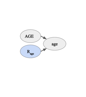
  Figure 2. The missingness indicator for "age" is completely independent of the data.
• 

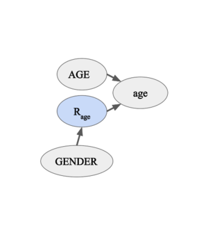
  Figure 3-1. The missingness indicator for "age" is dependent on the variable "GENDER" but not on the variable "AGE".
• 

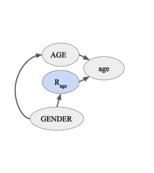
  Figure 3-2. The variable "age" is dependent on the variable "GENDER". However, the missingness indicator for "age" is conditionally independent of the variable "AGE" given the variable "GENDER".
• 

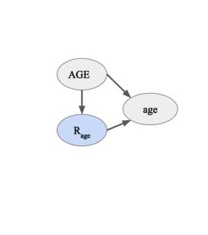
  Figure 4. The missingness indicator for "age" is dependent on the variable "AGE".

Table 1. An example survey form where the age column may have missing entries

Index	Name	Age	Occupation
1	John Doe	26	Construction worker
2	Dohyun Nam	?	Doctor
3	Mostafa Sharif	?	Graduate student
4	Jane Lee	17	High school student

• Scenario A, Figure 2. (MCAR): consider a scenario where the "Age" column in a survey form is missing due to pure chance. As noted in the previous section, $R_{age}$is an independent Bernoulli random variable with a fixed probability $p_{age}$such that $P(R_{age}=1)=p_{age}$. Then under the independent identical distribution (IID) assumption, the estimation of the overall distribution of age should not be affected by missing data.
• Scenario B, Figure 3-1 and Figure 3-2 (MAR): consider a scenario where the "Age" column in a survey form is missing because women are less likely to reveal their age, i.e. $P(R_{age}=1\ |\ GENDER=female)\neq P(R_{age}=1)$. In other words, the random variable $R_{age}$depends on the random variable "GENDER". Note that the variable "GENDER" does not need to be observed in the data. In this case, knowing the conditional probability $P(R_{age}=1\ |\ GENDER=female)$might useful, but inference does not require an explicit modeling of this probability [3]. In this scenario, semi-supervised learning approach such as expectation maximization can impute the missing age values without introducing further bias (given that there is sufficient amount of data).
• Scenario C, Figure 4 (NMAR): consider a scenario where the "Age" column in a survey form is missing because older people are less likely to reveal their age. In this case, $P(R_{age}=1\ |\ AGE=\alpha )$must be estimated, i.e. we must model why the data are missing.

Treatment of Missing Data

Depending on the missingness assumption and whether the data is complete during learning or prediction, one may or may not recover reasonable performance in the presence of missing data. In this section, we discuss imputation as a general technique to address missing entries in data and discuss some common imputation methods. We motivate a case for imputation using list-wise deletion as a baseline method.

List-wise Deletion

List-wise deletion refers to the deletion of examples or features that contain missing entries. For example, in Table 1., since the "Age" column is missing a the entries for examples 2 and 3, we can exclude those examples from analysis. This is a reasonable treatment under the MCAR assumption, assuming we have a sufficiently large number of IID examples, because the overall distribution of the data would not be affected by such deletions. However, MCAR is often an implausible assumption. If MCAR does not hold, then excluding examples and/or features will introduce bias in inference and learning, as the dataset will deviate from the true distribution. Hence, we will work with the MAR assumption and introduce imputation as an approach to treat missing data under such an assumption.

Imputation

Imputation refers to the technique of replacing the missing entries with the most likely values in their place. Imputation allows for maintaining the dimensionality of the data, while taking its missingness into account for doing inference. The specific strategies for imputation must take the missingness assumption into account. Choosing an imputation strategy that is based on an incorrect assumption can lead to increasing the bias of the inference model, which can negatively affect its performance.

In Table 2 below, we provide some example imputation methods corresponding to each missingness assumption.

Table 2. Imputation Methods

Assumption	Method	Description
MCAR	Mean Substitution	Replace each missing entry with the mean value of the corresponding feature
MCAR	Hot Deck	Replace each missing entry based on similar examples.
MAR	Expectation Maximization	Place an initial guess for missing entries and underlying parameters, e.g. $P(R_{j}=1|X_{ij*}=x_{ij*})$. Iteratively optimize expected log-likelihood.
NMAR	Collaborative Filtering	Extract principal components from available entries and reconstruct the original.

Classification with Missing Data Using Generative Model

Consider some datapoint $i$. Classification refers to the task of predicting the discrete response $y_{i}$ based on the observation $x_{i1},x_{i2},\cdots ,x_{id}$of the datapoint. With missing data, it is useful to limit our scope to inference with generative models, since there is no principled solution to this problem in discriminative models [2]. Generative models postulate the joint distribution $P(X_{i1},X_{i2},\cdots ,X_{id},Y_{i})$based on available and missing entries in order to answer probability queries such as $P(Y_{i}=y_{i}\ |\ X_{i1}=x_{i1})$. In his textbook, Murphy shows how a generative classifier may mitigate the missingness in data, depending on whether data is available or not at training time [2]. The discussion is summarized below.

Complete training data, incomplete test data

Here, incomplete data refers to data with missing entries. For example, Table 1 from the Examples section is incomplete because some of the "Age" entries are missing. Now, let us consider the case where the features in $X$are complete during training time and incomplete during test time. By incomplete, we imply that some of the features are missing. When these features of the test set are MAR, we can handle the missing entries via marginalization. Following the notations in the Preliminaries section. Consider computing the following probability:

$$P(Y_{i}=y_{i}\ |\ X_{i1}=?,X_{i2}=x_{i2},\cdots ,X_{id}=x_{id};\Theta )$$

As apparent, feature $X_{i1}$ is missing for the test datapoint. Then, assuming MAR, the best we can do is marginalize out $X_{i1}$and compute the following probability instead:

$$P(Y_{i}=y_{i}\ |\ X_{i2}=x_{i2},\cdots ,X_{id}=x_{id};\Theta )$$

Using the definition of conditional probability, we conduct the following steps:

$$={\frac {P(Y_{i}=y_{i},X_{i2}=x_{i2},\cdots ,X_{id}=x_{id};\Theta )}{P(X_{i2}=x_{i2},\cdots ,X_{id}=x_{id};\Theta )}}$$

$$={\frac {P(X_{i2}=x_{i2},\cdots ,X_{id}=x_{id}|Y_{i}=y_{i};\Theta )P(Y_{i}=y_{i}\ |\ \Theta )P(\Theta )}{P(X_{i2}=x_{i2},\cdots ,X_{id}=x_{id};\Theta )}}$$

$$\propto P(X_{i2}=x_{i2},\cdots ,X_{id}=x_{id}|Y_{i}=y_{i};\Theta )P(Y_{i}=y_{i}\ |\ \Theta )$$

Now, note:

• Since we have a complete training data, we can estimate $P(X_{i1}=x_{i1},X_{i2}=x_{i2},\cdots ,X_{id}=x_{id}\ |\ Y_{i}=y_{i};\Theta )$over the entire domains of the variables $X_{i1},X_{i2},\cdots ,X_{id},Y_{i}$. (1)

• $P(X_{i2}=x_{i2},\cdots ,X_{id}=x_{id}|Y_{i}=y_{i};\Theta )$is a result of marginalizing out over the domain of $X_{i1}$in the above conditional probability.

Which corresponds to this equality:

$$=P(Y_{i}=y_{i}\ |\ \Theta )\sum _{x_{i1}}P(X_{i1}=x_{i1},X_{i2}=x_{i2},\cdots ,X_{id}=x_{id}\ |\ Y_{i}=y_{i};\Theta )$$

For a Naive Bayes classifier, this computation reduces to conditional probability estimation.

$$=P(Y_{i}=y_{i}|\Theta )\sum _{x_{i}}P(X_{i1}=x_{i1}|Y_{i}=y_{i};\Theta )\prod _{j=2}^{n}P(X_{ij}=x_{ij}|Y_{i}=y_{i};\Theta )$$

$$=P(Y_{i}=y_{i}|\Theta )\prod _{j=2}^{d}P(X_{ij}=x_{ij}|Y_{i}=y_{i};\Theta )$$

Notice that this is equivalent to excluding the feature with missing entries from posterior calculation.

Incomplete training data, incomplete test data

When data is missing at training time, marginalization alone cannot treat missing data, as the joint conditional probability in (1) above cannot be estimated based on training data. Then computing the MLE or MAP estimate is no longer a simple optimization problem [2].

Conclusion

Handling missing data is very important. To avoid introducing further sources of error, it is important to reason about the process by which the data is generated, and to deduce the missingness pattern in the data. Identifying the correct missingness assumption and using an appropriate technique for treating missing data allows for an unbiased analysis despite missing entries.

Annotated Bibliography

1. Pearl, Judea, and Karthika Mohan. "Recoverability and testability of missing data: Introduction and summary of results." (2013).
2. Murphy, Kevin P. Machine Learning: A Probabilistic Perspective. Cambridge, MA: MIT Press, 2012. Print.
3. Mohan, Karthika, Judea Pearl, and Jin Tian. "Graphical models for inference with missing data." Advances in neural information processing systems. 2013.
4. Marlin, Benjamin. Missing data problems in machine learning. Diss. 2008.
5. Marlin, Benjamin M., et al. "Recommender systems, missing data and statistical model estimation." IJCAI proceedings-international joint conference on artificial intelligence. Vol. 22. No. 3. 2011.
6. Wikipedia contributors. "Imputation (statistics)." Wikipedia, The Free Encyclopedia. Wikipedia, The Free Encyclopedia, 4 Feb. 2019. Web. 5 Feb. 2019.
7. Rubin, Donald B. "Inference and missing data." Biometrika 63.3 (1976): 581-592.

To Add

• Testability of inference models with missing data
• Recoverability with missing data
• Causality with missing data