Course:CPSC522/Text Summarization for busy people!

Text Summarization: Tool for busy people

This article covers the final phase of text summarization where we practically see how can build a text summarizer and evaluate its efficiency and correctness. To gain more insights about text summarization and some previous work which aims to build a text summarizer using machine learning techniques, please have a look at the Text summarization using machine learning article. This article is built upon the previous article Text summarization using machine learning and explores how we can use Sequence-to-Sequence models to build an abstractive text summarizer. Sequence-to-Sequence models were used instead of decision trees or support vector machines as referred in the related work, mainly because today's state-of-the-art text summarizer are based on Sequence-to-Sequence model.
So, in your daily busy life, if you want to ease some hassle of going through an utterly long article and are looking for a smarter way to get information. Then keep on reading as this article, as it will provide all the details you should know to either build a text summarizer or use one.
Alas!! I wish I could summarize this article for you guys!!

Principal Author: Ekta Aggarwal

Abstract

This article gives a high-level idea of how - extractive and abstractive - text summarizers work. It then digs deeper into abstractive text summarizers and demonstrates how to build one. Finally, the results which are extracted from the system are shown and compared with similar techniques which work on abstractive summarizers.

Builds on

This article builds on the concept of Automatic Summarization and uses Sequence-to-Sequence model to create an abstractive text summarizer. Sequence-to-Sequence models internally use Long short-term memory LSTM to create summaries intelligently. Recurrent Neural Networks are an inseparable part of the Sequence-to-Sequence model and form the basis of many sequence-based inputs like videos(sequence of frames), text (sequence of words).

Background

Extractive v/s Abstractive Approach

As described in Text Summarization using Machine Learning, text summarization is a process of producing a short, concise and coherent text from the given input text. Text summarization can be achieved in two ways:

• Extractive - Here, the sentences or the phrases of the given input text are ranked by various algorithms. Then the ones which receive the highest score are chosen to become a part of the summarized text. Below are mentioned few of the extractive text summarization algorithms and implementations:

1. PyTeaser is a Python implementation, where features such as sentence length, title feature, sentence position and keyword frequency are used to rank the sentences.
2. PyTextRank is an improved implementation of the TextRank algorithm in Python which in this case ranks the sentences of the given input text.
3. LexRank is a graph-based approach based on TextRank.

Thus, an extractive technique is pretty easy as compared to the abstractive, as we just need to select important sentences from the given text. In the Text Summarization using Machine Learning article, the two papers that are referenced using extractive strategy to construct summaries.

• Abstractive - On the other hand, abstractive summaries are more challenging. Mainly because of the fact that they can use even those phrases/words which are not in the given input text. Therefore, a summarised text can contain words from the given input text and the vocabulary that the model builds. These summaries are ideally the ones that humans generate. The use of deep learning for building an encoder-decoder architecture for text summarization has lately been in the news. Top technology companies like Facebook, IBM, and Google have used encoder-decoder as the base of their text summarization algorithms.

1. The Facebook AI Research used a model that uses the encoder-decoder model with a convolutional neural network encoder. More information can be found in the paper

A neural attention model for abstractive sentence summarization written by their team.. Thier model can be found on the Github page detailing all the steps required to setup and run the summarizer on your local machine.

1. The IBM Watson model that uses the encoder-decoder model with pointing and hierarchical attention. The paper Abstractive Text Summarization Using Sequence-to-Sequence RNNs and Beyond . by their team dives deep into the architecture and working of their model.
2. The Stanford / Google model that uses the encoder-decoder model with pointing and coverage. Get To The Point: Summarization with Pointer-Generator Networks paper talks about the novel architecture that augments the existing sequence-to-sequence model. Their model can be found on the Github page.

Technically, encoder-decoder architecture is developed for Sequence-to-Sequence prediction. The use of Sequence-to-Sequence models, for text summarization, has taken the game to another level. For the purpose of the implementation of this article, Google's TensorFlow model was chosen, as there was prior knowledge about the platform. Google's text summarization model was trained to generate abstractive summaries using the first two lines of the news article. It was trained on Gigaword dataset which comes with a price!! The model gave good results after being trained on for a week with 4 million pairs from Gigaword dataset and using 10 machines with 4 GPU's each. Figure 1, shows some of the results achieved by Google's Brain Team. Notice the first example in Figure 1, the actual text doesn't contain the words "higher revenue", but they show up in the headline generated by the model. This shows that the model has learned how the semantics of the language work from all the input data which is given to it. Thus, it ended up in using a word/phrase which was in its vocabulary but not in the input text.

Figure 1: The image shows some results from the Google's TextSum models

Sequence-to-Sequence Models

Sequence-to-Sequence models as the name suggest converts a given input sequence to an output sequence. They contain two Recurrent Neural Networks(RNN), one called the encoder and the decoder. An RNN is a special type of neural network which is capable of using sequences/streams of data, for example, videos and text. A naive RNN is also called vanilla RNN and is pretty bad at remembering long sequences. So, to increase the capability of an RNN to work with long sequences of input, a more complex version called Long Short-term Memory (LSTM) is used. Sequence-to-Sequence models use two RNN's with LSTM cells to retain the information learned from the training data. For more details about RNN, please look at RNN article and RNN Wikipedia article. And LSTM's can be found on its wikipedia page. Figure 2 shows a basic Sequence-to-Sequence model with its basic building blocks - encoder and decoder.

Figure 2: Basic Sequence-to-Sequence model with LSTM encoder and decoder

In a nutshell, the Sequence-to-Sequence models work by creating a context from the given input sequence. This input sequence is then given to the decoder which ultimately converts it to the required output sequence. Some domains in which Sequence-to-Sequence models have been successfully applied using text as input are:

• Language translation - As can be seen in Figure 3, "hello how are you" is the input text sequence, to which the model produces a sentence which has the same meaning in another language. To attain this result, the model is trained with pairs of sentences from the input language and the output language. After the training is complete, the Sequence-to-Sequence model understands the context and use of words from the input language and thus construct a sentence which has the same meaning in another language. Additional information on how to create your own language translation model can be found on this blog.
  

  Figure 3: Sequence-to-Sequence model being used to convert a sentence in one language to the other.

• Auto-reply - While in Figure 4, the model can be seen to reply to the sentence given as the input, in the same language as the input. The model works on the input - a sequence of words or a sentence - to figure out the next word in the output one by one. The aim is to not lose any important information while being coherent with the input. More information on how to use Sequence-to-Sequence models for auto-reply can be found on this page.
  

  Figure 4: Sequence-to-Sequence model is given input a sentence and some response is expected from it in the same language.

• Text summarization - Glancing at Figure 5, we see that the input is a sentence which starts with "The United States became the largest tech..." is given to the encoder and it passes on the context derived from it to the decoder. This is a high-level view of the text summarizer, to know the detailed version of it, please keep reading.

Figure 5: Sequence-to-Sequence model being used to summarize the given input text sequence.

Hypothesis

As described above, the sequence-to-sequence model does not train on the whole article, but only on a partial one. Even Google's text summarization model was tested by feeding just first two lines of each text and generating headings out of it. This accomplishment can be considered the first step towards summarizing large documents of text. Thus, the hypothesis of this experiment is to vary the size of the input, from say 2 lines to 10 lines for each input document and see how the sequence-to-sequence model responds. With the current approach, it is hypothesized that with an increase in the input text, training time will increase and the summaries that will be generated will be less coherent with the given input text i.e. loss will not decrease at a faster rate.

Building a Text Summarizer

As described above, this article describes how to build a text summarizer using Sequence-to-Sequence models. Below is the detailed description of the various steps required to create the building blocks of text summarizer.

Data collection and Data preprocessing

Having a large set of data on which the model can be trained is of vital importance. Further, the data in the dataset should be clean and needs to be pre-processed to confirm its structural validity.
For text summarization, a dataset which contains articles with their human-generated headlines is required. The model is trained on the article's text to produce the headline as given in the text. As mentioned above, Google's TextSum was trained on Gigaword dataset which contains almost 10 million documents and comes with a price! So, instead of using Gigaword, a free source of data of articles and headlines was used, which contained almost 90,000 documents. Though the data set is not as elaborate as the Google's, it surely is a starting point.
After obtaining the dataset, it needed some cleaning mainly because of the following format that the Sequence-to-Sequence model needs:

• Special characters such as comma, full stop, question mark etc., are removed from the input article's text and the human-generated headline.
• All input sentences that are to be given to the model for training needs to be of the same length. So, to achieve this padding was added to the end of the sentence to make it of the desired length.
• The size of vocabulary is another tricky aspect of training the model. If the vocabulary is less, the summaries generated will not be of good quality, but if the vocabulary is huge, then it will take a lot of time to train and will definitely need more samples to learn the semantics of the language. So, to handle the large size of vocabulary, bucketing is used, where buckets of different sizes are created and the sentences are assigned a bucket according to its length.

Other than that, Sequence-to-Sequence model does not train on the whole article, but only picks up the first 2 lines of the article, to generate a heading out of it. The main reason for the use of just first 2 lines according to me is to simplify the whole text summarization. That is, to start out with a small section an then gradually build up to summarize the whole text. As can be inferred, if the Sequence-to-Sequence model is supplied the whole text, its input dimension will increase drastically, also increasing the size of vocabulary by many folds. And it would ultimately lead to usage of more resources such as a number of GPU's, memory, the time taken to train the model.
This approach was used by Google's Brain Team. So, to follow their footsteps, in this implementation, the length of the article has been restricted to 500 words and not the whole article.

Figure 6: A small part of CNN data set used to train Sequence-to-Sequence model

Figure 6, shows a small part of the CNN dataset which was used for training. It was pre-processed before being fed into the model. For preprocessing step, the article's text and the human-generated headline was trimmed to the desired length (500 for an article, while 50 for heading). Also, special characters were removed and sentences were lowercased and split into words by using space. To make all the sentences of equal length, they were padded. One important point to note here is that after this preprocessing step, we will have two bags of words, one for the article's text and another for the headline. Word to index and index to word mappings were created to better understand the semantics of the input. The vocabulary was generated using the words found in the article and headline. In the end, a mapping of words from the sentence is given to the encoder of the Sequence-to-Sequence model.

Let's see an example of how the data preprocessing step is done: In Figure 6, which shows a small subset of the input given to the preprocessing module, if we take the first line of the first input article's text, which is

Usain Bolt rounded off the world championships Sunday by claiming his third gold in Moscow as he anchored Jamaica to victory in the men's 4x100m relay.

Removing the special characters and lowercasing the above text, we get

usain bolt rounded off the world championships sunday by claiming his third gold in moscow as he anchored jamaica to victory in the mens 4x100m relay

Then tokenizing the above sentence, we get a bag of words, which are shown below

usain, bolt, rounded, off, the, world, championships, sunday, by, claiming, his, third, gold, in, moscow, as, he, anchored, jamaica, to, victory, in, the, mens, 4x100m, relay

At this point, we will create embedding of the bag of words specified above. In this step, we create a vector of fixed size, for example, 500 for this implementation. We will initially start with an empty vector of length 500, that is having "0" at all places

[0,0,0,0,0,........0,0,]  length = 500

Then using the tokenized words from above, we will update the vector of "0"'s, showing the number of times a word has occurred in the input text. So, just for illustration purposes, let assume that we get the following updated vector

[1,1,1,1,1,1,1,1,1,1,1,1,1,1,1,1,1,1,2,...,0,0,0] length = 500

Here, all the "1"'s depict that the word was encountered only once in the input. For example "usain" came only once, while "in" came twice which is shown by "2" in the vector. Word to index and index to word mappings are made for each of the tokenized words. This vector and the metadata is now fed into the encoder of the Sequence-to-Sequence model.
Pseudo-code for the data processing part used in this implementation is mentioned below:

function dataPreProcessing (articles, headlines):
  # "articles", contain list of articles in their raw form. That is, as found in CNN dataset.
  # "headlines", contain lists of headlines for each article in "articles" as found in CNN dataset.
  for each headline h in headlines:
     lowercase headline h
     tokenized = split the headline h by space (" ")
     get the length l of the tokenized array tokenized of words of the above headline h
     if length l > MAX_INPUT_HEADLINE_LENGTH:
        get the first MAX_INPUT_HEADLINE_LENGTH words from the tokenized headline tokenized, and update it
     maintain the count of occurrence of each word target_counter from the input tokenized array. 
     
  # repeat the above for loop with "articles" as the iterator, replace MAX_INPUT_HEADLINE_LENGTH with MAX_INPUT_ARTICLE_LENGTH and target_counter with input_counter
  # now its time to create the word-to-index and index-to-word dictionary and also the vocabulary of the model
  # using the above saved, target_counter, input_counter
  
  create an empty dictionary to store targetWord2Index data
  for each idx,word in target_counter:
      targetWord2Index [word[0]] = idx + 1
  
  # then do the above step for input_counter
  create an empty dictionary to store inputWord2Index data
  for each idx,word in input_counter:
      inputWord2Index [word[0]] = idx + 1
  
  return the tokenized articles, headlines, word-to-index and index-to-word dictionaries and also the vocabulary for the model to start training

Building a Sequence-to-Sequence model

After cleaning the data and preparing the vectorised representation of the input, now its time to start building the model to train. Google's Sequence-to-Sequence model is open sourced and is available in different implementations like TensorFlow, PyTorch, Keras etc. For this implementation, Keras was chosen mainly because of its ease of usability. Keras is a Python wrapper of TensorFlow, CNTK or Theano, which abstracts the lower level details of TensorFlow and provides easy to use API for machine learning purposes.

For the ease of understanding, let's take carry forward our example of using the first sentence from the first input given in Figure 6.

Figure 7: Structure of Sequence-to-Sequence model using the first input from training set

Just for visualization purposes, instead of having the vector containing the index of each word in the input article, we take the words themselves. Figure 7, shows an example of the structure of the Sequence-to-Sequence model using the first line of the first input training example. The first part is the encoder containing the orange nodes, while decoder is shown with blue nodes. As can be seen from the encoder in Figure 7, the output of the current hidden node is influenced by the current input word, like "bolt", "rounded" and the output of the previously hidden node. Similarly, the decoder hidden nodes use the response from the previously hidden node and the context which was passed from the encoder. To sum up this approach, it uses the words from the input to generate the output i.e summarised text one word at a time.
Using this approach, the Sequence-to-Sequence model can generate many versions of text summarizations, let us say k, out of which the best could be chosen. There are two techniques with which the best summary could be picked.

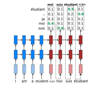
• Greedy search - As shown below, the decoder layer outputs a number of words which it thinks might be used as the first word of the output. Associated with every likely output are their probabilities. So, in greedy search, the algorithm picks the words which have the greatest probability that the other words. For example, for the first word outputted by the decoder, "moi" has the greatest probability of 0.4, thus gets selected and is served as the input for the second hidden unit of the decoder layer. This process is carried until it reaches the (end of the input). Thus, over here the search is greedy because it is picking only the best word out of all the possible ones.
  
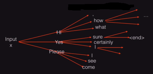
• Beam search - On the other hand, beam search is not that greedy and as shown in the figure below. Given the input X, it starts by computing different possible words that could be chosen for the first word of the decoder. This process up to here is similar to the greedy search. But now, instead of choosing the best one, the beam search algorithm carry forwards the process by putting each and every possible word as the input to the decoder's next node. It will ultimately lead to a tree-like structure and a lot of summaries which could be attained by traveling down the root node to the leaves. But in order to choose the best summary, it calculates the joint probability of each of the summary and then chooses the one which has the maximum.
  

For example, given the input X, the model will output the first word which it thinks is best suited for the summary. Then, it uses this first word and feedbacks into the model to generate suitable second word for the summary. This approach will lead to a tree-like structure where the root node is the input X, the first layer shows all the nodes which are deemed the best fit for the first word of the summary. Similarly, the second layer shows all the nodes that come after the first word of the summary generated. This tree will keep on growing as the number of words in the summary are increasing. In the end, many summaries will be generated by traveling each branch of the tree from root to the leaf. To choose the best summary from the available ones, beam search can be used. Beam search will calculate the joint probability of each possible summary and then choose the one with the maximum probability.
Some hyper-parameters which are to be kept in mind while working with Sequence-to-Sequence models:

• Maximum length of the vectorized input vector
• Maximum length of the vectorized output vector
• Maximum size of the vocabulary

The Pseudo-code below gives a high-level view of the implementation of the Sequence-to-Sequence model.

function buildSeq-to-SeqModel (preProcessedData):
  create encoder_inputs and an embedding layer for the encoder encoder_embedding using Keras API's.
  create encoder_lstm by using the above created embedding layer encoder_embedding
  
  # repeat the above steps for decoder also
  create decoder_inputs and an embedding layer for the decoder decoder_embedding using Keras API's.
  create decoder_lstm by using the above created embedding layer decoder_embedding
  set the hyper-parameters passed in the input of this function into the model
  use Kera's API to make the model using the encoder_lstm and decoder_lstm

Results

As described above, CNN data set was used for training and validating the Sequence-to-Sequence model. There were approximately 90,000 articles/documents in it with each having a headline. For this implementation, only 10,000 of the 90,000 documents were taken, because of the constraints of the machine on which the model was being trained. As there was no super-computer or a loaded GPU machine available, all the experimentation was done on a local machine with a GPU. Out of the 10,000 articles, the ratio of 4:1 was selected to partition the data. So, it ended up having 8,000 training examples and 2,000 validation examples.
Moreover, to show how the model is improving the number of epochs increase, the same validation set is chosen. This would help us better evaluate, the summary generated by the model after being trained for just 1 epoch and can be subsequently checked after 50 epochs, 100 epochs, and so on. For implementing the Sequence-to-Sequence model, Keras was used mainly because of developer friendly environment. As Keras internally refers to TensorFlow, so essentially Google's TextSum model is being used in this implementation. For the purpose of evaluating the hypothesis, the length of the input text is varied from 500 to 1000, that is it took 500, 750 and 1000 as the values for three individual experiments. For each experiment, the model was trained for 200 epochs and the time taken to train the model increased as the size of maximum vectorized input increased. It took around approximately 13 hours for 500 as the maximum length, while 18 hours for 1000 words as the maximum length. For each experiment, the loss incurred and accuracy gained over the training data set is reported with respect to the number of epochs. Also, the summaries that the model generated for each the experiments are shown below.

• The first set of hyper-parameters are:

1. Maximum length of the vectorized input vector - 500
2. Maximum length of vectorized output vector - 50
3. Maximum size of vocabulary - 5,000

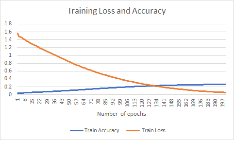
In this experiment, the maximum length of the vectorized input is kept to the minimum, that is 500. But one important point to note here is that in Google's implementation they kept it simple by just using the first two lines as the input. Thus, the maximum length of the input vector for their experiment can be approximated to 100 words. So, a reason to have approximately fivefold increased this hyper-parameter for this experiment is to judge how well the algorithm performs with large sets of the input text. From the figure above, we can see that during training the training loss decreased significantly from approximately 1.6 to 0.75 in just 200 epochs. And the accuracy increased from approximately 0% to 25%.

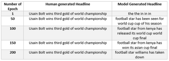
In the figure above, we can see how the model performs on the same input article by varying the number of epochs for which it was trained. After the first epoch of training, it produces random words. But as the number of epochs increases, the model learns and produces better results. One important point to take into account is that having trained for just 200 epochs is not enough to get the best performance from the model. But due to limited resources, a number of epochs were restricted to 200.

• The second set of hyper-parameters are:

1. Maximum length of the vectorized input vector - 750
2. Maximum length of vectorized output vector - 50
3. Maximum size of vocabulary - 5,000

Notice that the maximum length of the vectorized input has been changed for this experiment. Initially, it was set to 500, but now to evaluate the hypothesis it is set to 750. This change will help us judge what effect does the length of vectorized input have on qualities of summary generated.

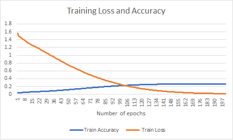
From the above figure, we can see that during training the training loss decreased significantly from approximately 1.566 to 0.0157 and the accuracy increased from approximately 3.65% to 26.64%. These figures are slightly better than the previous results where we were using 500 as the length of the vectorized input.

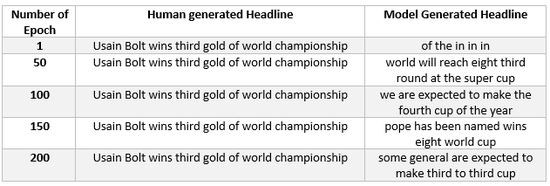
The figure above shows the result obtained from the model on the same headline, as was used in the above experiment. We can see that the summaries that are generated have changed, but still, they are not comparable to the headlines generated by the humans.

• The third set of hyper-parameters are:

1. Maximum length of the vectorized input vector - 1000
2. Maximum length of vectorized output vector - 50
3. Maximum size of vocabulary - 5,000

In this experiment, the maximum length of vectorized input was changed to 1000 and the model was trained from scratch for 200 epochs. The results are shown below.

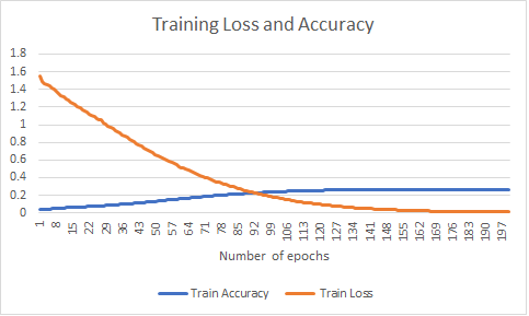
The graph above shows how training loss and accuracy vary with as the number of epochs increase. The loss begins with a value of 1.555 and reduces to 0.009. The value of loss attained in this case after 200 epochs are the least when compared to the above two experiments. While the accuracy of the trained model, it increased from 3.72% to 26.66% which is around the value attained for the above two experiments.

In the above table, showing the result for generating the headline after training the model for a specified number of epochs, we can see that different words were used/incorporated in the summary generated by the model. This effect could possibly be because of the increase in the length of input vector for this experiment. Though new words have been chosen for this summary, it doesn't seem the case that the summary generated by the model is coherent with the input article.
To summarize, using the current approach the increase in the length of the input articles does not give much of improvement in the headlines generated. This result is consistent with the hypothesis stated above.