Course:CPSC522/Image Classification With Convolutional Neural Networks

Image Classification with Convolutional Networks

Author: Surbhi Palande

Primarily referencing

Paper 1: ImageNet Classification with Deep Convolutional Neural Networks by Alex Krizhevski et al (2012).

Paper 2: Visualizing and Understanding Convolutional Networks by Matthew D Zeiler et al (2013): 147.

Principal Author: Surbhi Palande

Abstract

Since 1980s neural networks have attracted the attention of the machine learning and AI community. Yan Lecun’s landmark paper on “Gradient-Based Learning to Document Recognition” spearheaded the application of CNNs for character recognition. It compares the performance of several learning techniques on benchmark datasets. We first present a short description of CNNs from this paper. This is the basis on which we look at the actual papers.

The first paper that we look at, is widely regarded as an influential paper that brought attention back to using CNNs for image recognition. The authors Alex Krizhevsky et al created a “large, deep convolutional neural network” that shockingly won the 2012 ILSVRC (ImageNet Large-Scale Visual Recognition Challenge) with an accuracy of 85%. This was the first time that CNN was used to outperform other classification methods by a factor of 2. We look at this paper to study the architecture of the underlying CNN.

Despite achieving the success that it did, the working of CNNs was pretty much haphazard and based on trial and error. The CNN community lacked the intuition and understanding of what the CNN was actually doing. In 2013, Matthew Zieler et al wrote a paper on Visualizing and Understanding Convolutional Networks. In this paper, the authors give an intuition of what the network does and also thus provides ways to optimize its performance. This is the second paper that we look at.

Builds On

http://wiki.ubc.ca/Course:CPSC522/Convolutional_Neural_Networks

Related To

• http://wiki.ubc.ca/Course:CPSC522/Deep_Neural_Network

Background Knowledge

If you already know what CNNs are, skip here

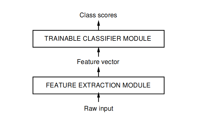
History of CNN

The usual method of recognizing individual patterns consists of dividing the system into two main modules shown in fig 1 The first module, called the feature extractor, transforms the input patterns so that they can be represented by low dimensional vectors or short strings of symbols that:

• Can be easily matched or compared AND
• Are relatively invariant with respect to transformations and distortions of the input patterns that do not change their nature.

The feature extractor contains most of the prior knowledge and is rather specific to the task. It is also the focus of most of the design effort because it is often entirely handcrafted. The classifier, on the other hand, is often general-purpose and trainable. One of the main problems with this approach is that the recognition accuracy is largely determined by the ability of the designer to come up with an appropriate set of features.

With the advent of low-cost machines, large databases and powerful machine learning technique - one could rely more on brute force numerical methods than on feature extraction algorithmic refinements. While more automatic learning is beneficial, no learning technique can succeed without a minimal amount of prior knowledge about the task. In multilayer neural networks, a good way to incorporate knowledge is to tailor its architecture to the task. Convolutional Neural Networks (aka CNN) are an example of specialized Neural Network Architectures. Convolutional networks are designed to learn to extract relevant features directly from pixel images. In the late 1900s, convolutional networks were usually trained by using the gradient descent based techniques. The surprising usefulness of such a simple gradient descent technique for complex machine learning tasks was not widely realized until the following three events occurred:

• Identification that local minima do not affect the calculations
• Simple and efficient application of this method to nonlinear systems
• Demonstration that Back propagation method + sigmoid classification solves complex learning tasks.

Once this happened, CNNs were again thought of as a reality.

What is a CNN?

Convolution neural networks or convnets or CNNs are neural networks that extract features from an input image. The process of extracting features is called as convolution. Quite naturally a CNN has atleast one convolution layer and one fully connected (FC) classification layer. Of course there can be multiple convolution layers and multiple FC layers. The input to a CNN consists of an image that has the dimensions such as width * height * depth where depth can represent R, G, B channels. The output of the CNN is a label classification of the image in terms of probability.

A typical convolution network for recognizing characters is shown in LeNet-5 which is one of the early CNNs

. The input plane receives images of characters that approximately are size normalized and centered.

In general, Convolutional networks combine three architectural ideas to ensure some degree of shift, scale and distortion invariance:

• Local receptive fields
• Shared weights
• Spatial or temporal subsampling.

Each unit in a layer receives input from a set of units located in a small neighborhood in the previous layer. With local receptive fields, neurons can extract elementary visual features such as oriented edges, end-points, corners, surrounding etc. These features are then combined/condensed into high-level features. Units in a layer are organized in planes within which all units share the same weights. The set of outputs of the units in such a plane is called a feature map. Units in a feature map are all constrained to perform the same operation on different parts of the image. A complete convolution Layer is composed of several feature maps (with different weight vectors). Each pixel participates in the extraction of multiple features.

So each plane is a feature map. A unit in a feature map has n*n inputs connected to a n * n area (of neurons) in the input. This input is called as the Receptive field . Each unit has $n^{2}$ inputs and hence $n^{2}$ trainable coefficients plus a trainable bias. Receptive fields of neighboring units overlap. The amount with which each receptive field is moved to process the next set of input, is called as the stride. All the units in one feature map share the same set of $n^{2}$ weights and the same bias so they detect the same feature at all possible locations on the input. The other feature maps in the layer use different weights and biases thereby extracting different types of local features. In LeNet5 at each input location, six different types of features are extracted by six units in identical locations in the six feature maps. A sequential implementation of a feature map would scan the input image with a single unit that has a local receptive field, and store the states of this unit at corresponding locations in the feature map. This operation is equivalent to a convolution , followed by an additive bias and squashing function, hence the name convolutional network. In order to retain the information along the boundary of the image, during convolution zero padding is done on the image. This way the output of the convolution remains equal to the input of the convolution.

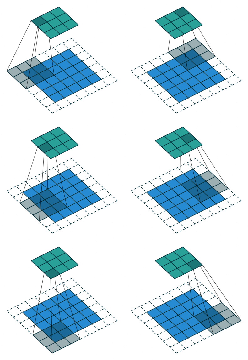
The kernel of the convolution is the set of connection weights used by the units in the feature map. An interesting property of the convolutional layers is that if the input image is shifted, the feature map output will be shifted by the same amount, but will be left unchanged otherwise. This property is at the basis of the robustness of convolutional networks to shift and distortions of the input.

The actual precise position of a feature is irrelevant. It is more important to find the position relative to the other features. Eg: While recognizing digits, if you find the endpoint of a roughly horizontal segment on the left corner, a corner in the upper right corner and the endpoint of a roughly vertical segment in the lower portion of the image, we can tell the input image is a 7. It is in fact potentially harmful to find the precise position of these features. A simple way to reduce the precision is through sub-sampling of layers - i.e perform a local averaging and subsampling to reduce the resolution of the feature map. This reduces the sensitivity of the output to shifts and distortions. The next layer is a subsampling layer. The input neurons still is a matrix, but it is nonoverlapping. Consequently, the output is condensed. This layer is used either to “blur” the input or add “noise” to the input. Successive layers of convolutions and subsampling are typically alternated, resulting in a bi-pyramid: at each layer, the number of feature maps is increased as the spatial resolution is decreased. This achieves a large degree of invariance to geometric transformations of the input. In some layers, the output feature maps can have inputs from receptive fields in several input feature maps. Subsampling can also be referred to as pooling. The most commonly used pooling function is a max-pooling function.

All weights are learned with back propagation. CNNs are seen as synthesizing their own feature extractor.

Supervised vs Unsupervised CNN

When a labeled dataset is used for training a CNN, the CNN can be called as a supervised CNN. This is mostly used for image recognition, classification etc. On the other hand when the training data is not labeled then the CNN is termed as Unsupervised CNN. This is mostly used for making an inference from the given data Eg: Image match, weather forecast etc.

Image Classification with CNNs

ImageNet Classification with Deep Convolutional Neural Networks

ImageNet Classification with Deep Neural Networks

Fast GPUs, fast 2D convolution, and availability of large databases of labeled images like ImageNet have made it possible to apply CNNs to high-resolution images. ImageNet consists over 15 million labeled high-resolution images. The images are collected from the web and labeled by human labelers using Amazon’s Mechanical Turk crowdsourcing tool. The specific contributions of this paper are:

• Trained one of the largest CNN on the subset of Imagenet images.
• Achieved best results ever reported
• Wrote a highly optimized GPU implementation of 2D convolution and all other operations inherent in training convolutional neural networks
• Introduces new and unusual feature in the CNN to improve performance and reduce training time
• Use several techniques to prevent overfitting

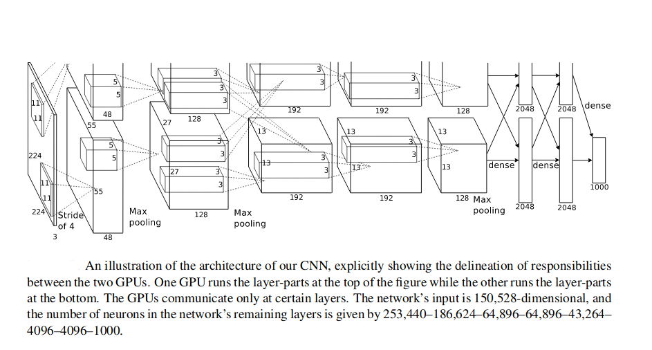
The network was trained on two GTX 580 3GB GPUs. The figure on the right depicts the CNN architecture. It contains 8 learned layers - 5 convolutional and 3 fully connected. As described in the link that explains CNN, the convolutional layers extract features from the image. The fully connected layers use these features to provide a classification of the image.

The output of the neurons is modeled using a tanh function $f(x)=tanh(x)=(1+e^{-x})^{-1}$. Based on this paper by "Nair and Hinton", the activation function was changed to ReLU. The authors found out that tanh is slower than using the ReLU function. Thus the training was accelerated by using ReLU instead of tanh. Another advantage of using ReLU is that it does not need input normalization to prevent them from saturating. Even if some training examples produce a positive input to ReLU, learning will happen in that neuron. Despite this property, input was “brightness normalized”. This normalization reduced the test error rate by 1.4% and 1.2% respectively for top-1 and top-5 error rate.

Overlapping pooling was utilized in the architecture to further reduce the top-1 and top-5 error rates by 0.4% and 0.3% respectively. In general pooling layer can be thought of as consisting of a grid of pooling units spaced s pixels apart. Each pooling unit summarizing a neighborhood of size z*z centered at the location of the pooling unit. In general pooling layer, s = z. However, the authors found out that settings < z, called as overlapping pooling, reduced the error rates.

In order to train the 1.2 million images, two GPUs were used inside of one machine. Half of the kernels are put on one GPU and the other half is employed on the other GPU. By doing this on multiple GPUs the framework did not have to reduce its number of kernels. Training on two GPUs was slower than training on one. However, the error rate was reduced.

Since this neural network architecture has 60 million parameters, without any proactive measure, the sheer number of parameters causes overfitting. Two models were employed to reduce overfitting in AlexNet:

• Data Augmentation
• Dropouts

Data Augmentation : The images in the dataset are artificially enlarged using label preserving transformations. This transformation of a new batch of images is done in parallel to GPU processing of previous images. Thus in terms of time, they are basically free. Two separate schemes are employed: Extracting “random” 224 * 224 patches from the original 256 * 256 images. 5 such patches were made by selecting the 4 corners and their center. The horizontal reflection of these gave another 5 patches. The prediction was made by averaging the prediction on these 10 patches. The RGB intensities in the images were altered. The principal component analysis is performed on the set of RGB pixel values throughout the ImageNet training set.This scheme approximately captures an important property that object identity is invariant to changes in intensity and color of the illumination. This scheme reduces top-1 error rate by 1%

Other than data augmentation, the second scheme used to avoid overfitting is Dropouts . Dropouts consist of setting to zero the output of each hidden neuron with a probability of 0.1. The neurons which are dropped out this way do no contribute to the forward pass and do participate in the backpropagation. So every time an input is presented, the neural network ends up sampling a different architecture. This is similar to combining the training results from different models., except that it is cheaper as the models/architectures now share weights. In order to implement dropouts, Alexnet employs the following scheme: The output of all the neurons is multiplied by 0.5. Dropouts are used in the first two fully connected layers. Without dropouts, the network exhibits substantial overfitting.

Learning was employed using stochastic gradient descent with a batch size of 128 examples, momentum of 0.9 and weight decay of 0.0005. Note that the very small weight decay results in the reduced training error. The update rule for the weight w was:

$v_{i+1}=0.9*v_{i}-0.0005*\epsilon *w_{i}-\epsilon *({\frac {dL}{dw}}|w_{i})$

$w_{i+1}=w_{i}+v_{i+1}$

The initial weights were chooses from a zero mean Gaussian distribution with standard deviation of 0.01. The neuron biases in the second, fourth and fifth convolutional layer was set to 1. This initialization accelerates the early stages of learning by providing the ReLUs with positive inputs. The neuron biases in the rest of the layers were set to 0. The learning rate for all the layers was equal and was adjusted “Manually” throughout training. The training took place for nearly 5 days and was completed in 90 cycles of going through all the images.

The problem

Despite achieving the success that it did, the working of CNNs was pretty much haphazard and based on trial and error. The CNN community lacked the intuition and understanding of the internal working of CNNs or how they achieve such great performance. In 2013, Matthew Zieler et al wrote a fascinating paper on Visualizing and Understanding Convolutional Networks. In this paper, the authors give an intuition of what the network does and also thus provides ways to optimize its performance. This is the second paper that we look at.

Visualizing and Understanding Convolutional Networks

This paper introduces a visualization technique that reveals the input stimuli that excite individual feature maps at any layer in the model. It also allows us to allow the evolution of feature maps during training and to diagnose potential problems with the training. The visualization technique proposed is a Deconvolutional Network (deconvnet) to project the feature activations back to pixel space. This helps in understanding what pixels divulge what features, what layers study what features etc. This work first started by visualizing AlexNet and then improving its performance by changing the parameters such size of the receptive field, stride size etc. The generalization ability of the model to other datasets is then explored.

Related Work: Though visualization of convolutional networks has been done before, it has been applied to the first layer mostly. The exploration of the higher layers is done by few and restricted to a parametric invariance view. This paper, on the contrary, looks at the nonparametric invariance, showing which patterns from the training set activate the feature map. The uniqueness of this work is that it provides a top-down projection that reveals structures that stimulate a particular feature map.

Approach:

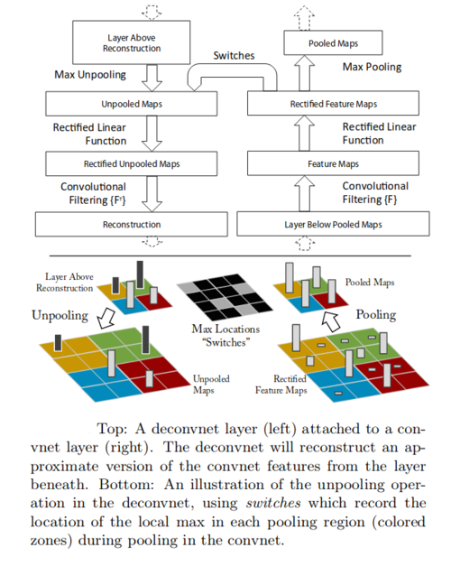
Understanding the operation of a convnet requires interpreting the feature activity in intermediate layers. Deconvnets are used for reverse mapping the features back to the input space. Thus a deconvnet can be thought of as the convnet model that uses the same components(filtering, pooling) in reverse. In this work, deconvnets are used as a probe of an already trained convnet. To examine a convnet, a deconvnet is attached to each of its layers as illustrated in the figure on the right. To examine a given convnet activation, we set all the other activations in the layer to zero and pass the feature maps as the input to the deconvnet. Then we successfully 1) unpool 2) rectify and 3) filter to reconstruct the activity in the layer beneath that gave rise to the chosen activation. This is then repeated until pixel space is reached.

• Unpooling: Since the maxpooling layer is irreversible, the location of the maxima is recorded. This is then used while unpooling to regenerate an approximate inverse where the structure of the stimulus is preserved.
• Rectification: The CNN uses ReLU nonlinearities, which rectify the feature maps thus ensuring that feature maps are always positive. The inverse of the ReLU function is the ReLU function. It sounds a bit odd, but the authors' argument is that since convolution is applied to rectified activations in the forward pass, deconvolution should also be applied to rectified reconstructions in the backward pass. Thus, to obtain valid feature reconstructions at each layer, the reconstructed signal is passed through ReLU nonlinearities.
• Filtering: The convnet uses learned filters to convolve the feature maps from previous layers. To invert this, the deconvnet uses a transposed version of the same filter but applied to rectified maps

Since unpooling uses recorded information of the local maxima, this is dependent on a particular image structure. The reconstruction obtained from a single activation resembles a small piece of the original input image with structures weighted according to their contribution to the feature activation. The model is trained discriminatively i.e certain pixels contribute to certain features which contribute to label classification. Thus deconvolution also shows which part of the input image are discriminative.

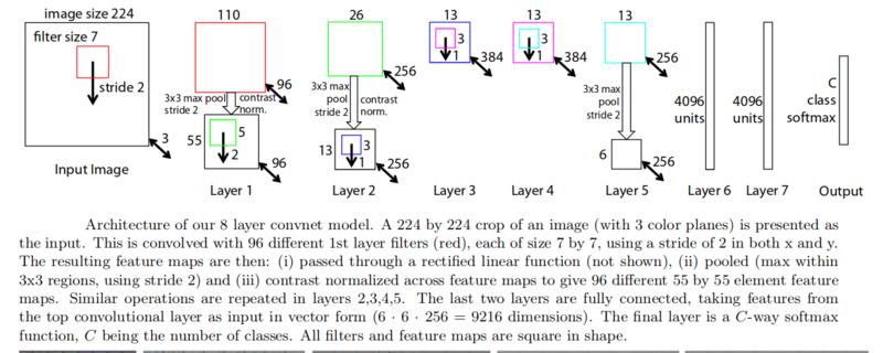
The architecture described in the first paper above is used for visualization. One discrimination is that in Krizhevsky’s model the layers 3, 4, 5 use sparse connections, whereas in here dense connections are used. For training, the same data as paper 1 was used - 1.2 million training images from ImageNet database. As in the first paper, the stochastic gradient was used for learning with a mini-batch size of 128 images, learning rate of 10^-1 and a momentum of 0.9. Like before the learning rate was manually annealed.

Convnet Visualization:

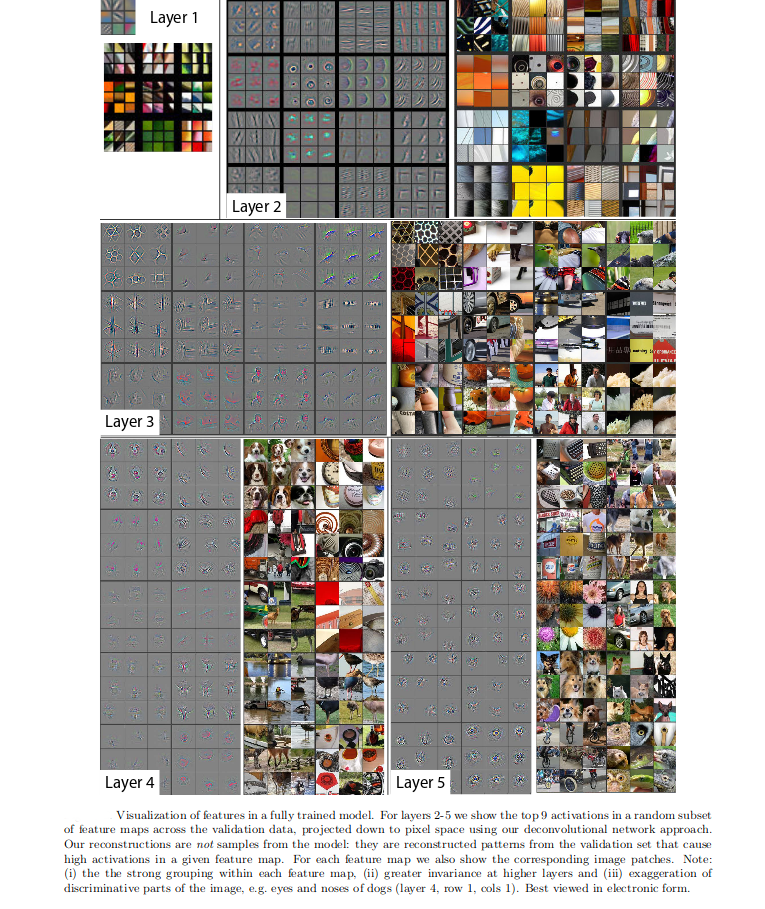
Fig above shows feature visualizations. Instead of showing the single strongest activation for a given feature map, this work shows the top 9 influential feature maps. Going from features to pixels shows what pixel structures affect what features.

Fig above shows feature evolution of the strongest activation during training across all examples. Lower (or the initial) layers of the model can be seen to converge in fewer epochs than the upper layers.

Visualization was also done by translating, rotated and scaling the training images by varying degrees. Comparing the features extracted from these transformed images with those of the original images shows that the first few layers are more sensitive to change and exhibit dramatic effects to smaller change. But the feature maps in the later layers seem to be quasi-linear to translation and scaling (not rotation). In general, the output seems to vary with rotation if the images lack rotational symmetry.

Analysis of the Krizhevsky Model in the first paper using this technique shows the following:

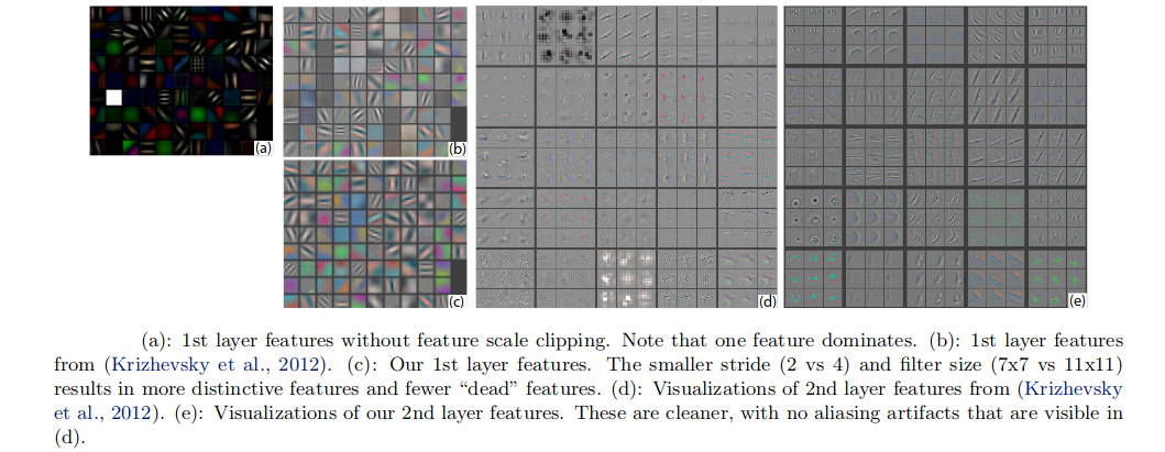
• The first layer filters are a mix of extremely low and high frequency information. Mid frequencies have little coverage.
• The 2nd layer visualization shows aliasing artifacts caused by a large stride 4 used in the first convolution layer. Aliasing causes smooth curves and other lines become jagged because the resolution of the image is not high enough to represent a smooth curve. Distinguishing features is harder because of this.

• Changing the stride to 2 and the size of the receptive field to 7 * 7 instead of 11 * 11, gave much better classification performance and retains better information in the first and the second layer. This is shown in the figure above.

In general, a stable model for image classification/recognition is not location dependent but rather makes sense of the image depending on its surroundings. Thus we need to make sure that enough surrounding is studied and that location-specific recognition is reduced. This is verified by occluding certain random portions from the image and monitoring the output of the classifier. When the occluder covers the image region that is included in the feature map, a strong drop in the activity of the feature maps is seen. This shows that visualization does correlate with the image structure. This validates the findings from the previous visualization images.

It is very interesting to study if CNNs implicitly learn the explicit mechanism for establishing a correspondence between specific object parts in different images. The paper mentions doing this not by using deconvnet, but by a technique such as calculating the difference between features from the original image and features from an occluded image. This difference is calculated for very similar images and then the difference is compared. The more similar the difference is the more correspondence between the occluded part and the features.

Algorithm 1 : Learning a single layer of the Deconvolutional Network

Require: Training images y # feature maps K, connectivity g
Require: Regularization weight λ, # epochs E
Require: Continuation parameters: β0, βInc, βMax
Initialize the feature maps and filters z ∼N (0, ε), f∼N (0, ε)
for Epoch = 1: E do
  for iteration = 1: I do
    β=β0
    while β < βmax do
    Given convolutional matrix solve for input</math> 
     β =β·βinc
    end while
end for
Update filter f using gradient descent.
end for
Output: filters f

Future Direction

CNNs take a very long time to train. Recently there has been a lot of work on optimizing training of CNNs. Facebook came up with a solution of training their ResNet-50 CNN in one hour time - which is a huge improvement over the previous work. There has also been work on improving the accuracy of training using different algorithms to correct the weights and to improve feature extraction. This seems like the general direction of research in CNN used for image classification.

To Add

Condensed evaluation from paper 1