Course:CPSC522/Convolutional Neural Networks

Convolutional Neural Network

Convolutional Neural Network (CNN) is a type of feed-forward artificial neural network, which has wide application in image and video recognition, recommender systems and natural language processing.

This page is based on:

1. Convolutional networks for images, speech, and time series.

2. Best practices for convolutional neural networks applied to visual document analysis.

3. Wikipedia: convolutional neural network.

4. Stanford cs231n course notes.

Author: Yan Zhao

Abstract

Convolutional Neural Networks (CNNs) are a type of feed-forward artificial neural network, which is designed to process image data. The idea of CNNs is popular in research community, but it is not that popular in engineering community until recent years. The reason might be the complexity of implementation. This page present some background information of CNNs based on paper of LeCun et al. , wikipedia and Stanford cs231n course notes . And then describe some practices of implementing CNNs proposed by Simard et al. to address the complexity of CNNs implementation.

Build on

Artificial Neural Network provides enough background information for this page.

Basics

Convolutional Neural Networks (CNNs) are very similar to ordinary Neural Networks (NNs). However, the architectures of CNNs are designed for image inputs. Therefore CNN have some special features that make the implementation more simple and efficient.

Overall Features

Ordinary NNs can be used for image recognition. However, the fully connectivity structures don't scale well to larger or higher resolution images. For example, images of size 200x200x3 (200 wide, 200 high, 3 color channels) will lead to 200*200*3 = 120,000 weights. The problem of ordinary NNs is that they treat each input pixel as an isolated data point, ignoring the spatial structure of image data.

CNNs are designed to emulate the behavior of a visual cortex, and can capture the spatially structures in images. The following features jointly allow CNNs to achieve better performance on image data:

1. 3D volumes of neurons. The layers of a CNN have neurons arranged in 3 dimensions: width, height, depth. This architecture takes advantage of the fact that inputs are images, which also have 3 dimensions: width, height, color channel.
2. Local connectivity. The neurons inside a layer are only connected to a small region of the layer before it, called a receptive field. CNNs can exploit spatially local correlation by enforcing such a local connectivity pattern.
3. Shared weights. In CNNs, each learnt pattern is replicated across the entire visual field by sharing the same parameterization. This grant CNNs the property of translation invariance.

The following figure shows the difference between ordinary NNs and CNNs.

Left: A typical 3-layer Neural Network. Right: A typical Convolutional Neural Network.

Building Layers

Layers are the basic building blocks of CNN architectures. Most commonly used layers includes:

Convolutional Layers

An example of convolutional layer. Note that there are multiple neurons (5 in this example) along the depth, all connected to the same local region in the input.

The convolutional layer is the core part of CNNs. Its output volume can be interpreted as neurons arranged in a 3D volume. And its parameters are set of learnable filters. Each filter is connected only to a local region in the input volume spatially (width and height), but to the full depth.

During the forward pass, each filter applied to a small local region, computing the dot product between the filter and the input. Then it iterate across the width and height of the input volume. The result of each filter is a 2-dimensional activation map. In this way, the network learns filters that activate when they see some specific type of feature at some spatial position in the input.

Stacking the activation maps for all filters along the depth dimension gives the full output volume of the convolution layer. Every entry in the output volume can thus also be interpreted as an output of a neuron that looks at a small region in the input and shares parameters with neurons in the same activation map.

Pooling Layers

An example of (max) pooling layer.

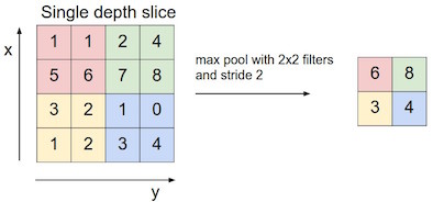
The pooling layer is another important part of CNNs. It is a form of non-linear sub-sampling. Pooling partitions the input image into a set of non-overlapping rectangles and, for each such sub-region, outputs the maximum (or average, L2 norm etc.). The intuition is that once a feature has been found, its exact location isn't as important as its rough location relative to other features.

Pooling layer will significantly reduce the size of input and also the amount of parameters and computation in the network. As a result, overfitting would not be a serious issue.

ReLU Layers

Rectified Linear Units (ReLU) layers apply non-saturating activation function $f(x)=\max(0,x)$. ReLU layers increase nonlinearity of the overall architecture without affecting the receptive fields of the convolution layer.

Other types of activation function also increate nonlinearity, such as the sigmoid function $f(x)=(1+e^{-x})^{-1}$. However, ReLU will lead to faster training without significant loss of accuracy. So ReLU is more commonly used in CNNs.

Fully-connected Layers

Fully-connected layers are usually the last layer of the overall architecture. They have full connections to their previous layers, just the same as the regular layers in ordinary NNs.

Architectures

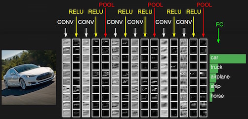
A CNN architecture is formed by a stack of several different layers. And there are some common patterns of layers stacking:

• Input -> Convolutional -> ReLU -> Full-connected
• Input -> [Convolutional -> ReLU -> Pooling] * 2 -> Full-connected -> ReLU -> Full-connected

The following figure gives a CNN architecture for image recognition.

An example of CNN architecture.

Best Practices

The idea of CNNs has been popular in research community for year. However, it is not that popular among engineering community until recent years. The reason may be the complexity of implementation and computational cost. In the paper of Patrice et al., the authors proposed two best practices (at that time) for implementing CNNs. Their experiments achieved best performance (at that time) for visual document analysis on MNIST data set.

Simple Loop for Convolution

Ordinary NNs often implement forward and backward propagation using the following rules:

$x_{j}^{L+1}=\sum _{i}{w_{j,i}^{L+1}x_{i}^{L}}$

$g_{i}^{L}=\sum _{j}{w_{j,i}^{L+1}g_{j}^{L+1}}$

where $x_{i}^{L}$ and $g_{i}^{L}$ are the activation and the gradient of unit $i$ at layer $L$, and $w_{j,i}^{L+1}$ is the weight connecting unit $i$ at layer $L$ to unit $j$ at level $L+1$. This can be seen as the activation units of the higher layer "pulling" the activations of all the units connected to them. And the gradients pull from the lower layer in similar ways. This pulling strategy is painful and complex to implement.

To simplify computation, we can instead "push" the gradients from upper layer. And the rule is:

$g_{j+i}^{L}+=w_{i}^{L+1}g_{j}^{L+1}$

This pulling strategy can be slow. But for large CNNs, it is negligible due to memory access pattern. But this strategy greatly reduce the complexity of implementation. From an implementation view, pulling the activations and pushing the gradients is the best strategy that achieves both simplicity and efficiency.

Modular debugging

Back-propagation allows NNs to be expressed and debugged in a modular fashion. Assume that a module $M$ has a forward propagation function which computes its output $M(I,W)$ as a function of its input $I$ and parameters $W$. Using the backward propagation function and gradient function, we can compute ${\frac {\partial I}{\partial M(I,W)}}$ and ${\frac {\partial W}{\partial M(I,W)}}$ by simply feeding the unit vector $\bigtriangleup {M_{k}(I,W)}$ to both of them. Conversely, we can estimate ${\frac {\partial M(I,W)}{\partial I}}$ and ${\frac {\partial M(I,W)}{\partial W}}$ by first-order difference approximation.

We also have equalities:

${\frac {\partial I}{\partial M(I,W)}}=F({\frac {\partial M(I,W)}{\partial I}})^{T}$

${\frac {\partial W}{\partial M(I,W)}}=F({\frac {\partial M(I,W)}{\partial W}})^{T}$

where F is a function which takes a matrix and inverts each of its elements. Based on these, we can verify whether the forward propagation accurately corresponds to the backward and gradient propagations. This simple debug strategy can save a significant amount of implementation time.

Results

The authors conducted several experiments on MNIST data set, and compared their results with some previous work. The results are listed below.

Algorithm	Distortion	Error	Ref.
2 layer MLP (MSE)	affine	1.6%	LeCun et al.
SVM	affine	1.4%	Decoste et al.
Tangent dist.	affine+thick	1.1%	LeCun et al.
Lenet5 (MSE)	affine	0.8%	LeCun et al.
Boost. Lenet4 (MSE)	affine	0.7%	LeCun et al.
Virtual SVM	affine	0.6%	Decoste et al.
2 layer MLP (CE)	none	1.6%	this paper
2 layer MLP (CE)	affine	1.1%	this paper
2 layer MLP (MSE)	elastic	0.9%	this paper
2 layer MLP (CE)	elastic	0.7%	this paper
Simple conv (CE)	affine	0.6%	this paper
Simple conv (CE)	elastic	0.4%	this paper

The distortion indicates type of pre-processing.

As we can see, the last entry (CNN with elastic distortion) of the above table achieves the best result. This illustrate the power of CNNs.

Summary

As proposed by LeCun et al. , CNNs can be a good idea for learning from various data including images, speech and time-series. However, the complexity of implementation was the bottleneck of its development. Therefore, both research and engineering communities proposed various tips and best practices for implementing CNNs, including the contribution of Simard et al. . They introduced the idea of a simple loop for convolution and modular debugging, which significantly reduced the implementation complexity of CNNs. And their experiments on MNIST data set showed that CNNs is one of the best techniques for visual document analysis.

The incremental contribution here is that the second paper proposed an efficient implementation of the idea from the first paper.