Black-Box Optimization using Bayesian Optimization

Title

Bayesian Optimizing aims to optimize black-box" functions which are difficult to model mathematically or are expensive to evaluate.

Principal Author: Mayank Tiwary

Abstract

BO aims to optimize an objective associated with a black-box function. The optimization process initially learns the behavior of the black box functions (using a surrogate model) by experimenting with different input values and observing the system's output. Once the learning is complete (the surrogate model gets trained), the optimizer predicts inputs that can maximize or minimize the objectives accordingly. As this is an interactive process where BO learns while experimenting, it is necessary to trade-off between exploration and exploitation. More exploration will generate more training data for better training of the surrogate model. As explorations can be expensive, Optimizer must understand when to stop further exploring and exploit what the surrogate model has already learned. Hence, to trade off between exploration and exploitation, BO uses an acquisition function.

Builds on

Bayesian optimization builds on Bayesian Inference, a statistical method for updating beliefs or probabilities based on new data. It uses this framework to model the trade-off between exploration and exploitation of a target function to efficiently find its global optimum. While Reinforcement Learning and Bayesian Optimization approaches have the goal of finding the optimal solution, they differ in the nature of the problem they are trying to solve and the methods they use to solve it. Bayesian Optimization is a method for optimizing black-box functions, which are functions where the information about the function, such as gradient or Hessian, is not available. It is mainly used for hyperparameter tuning in machine learning algorithms. Whereas, Reinforcement Learning, on the other hand, is a subfield of machine learning that focuses on decision-making in an environment where the agent interacts with its surroundings and receives feedback in the form of rewards. The goal is to find the optimal policy, which is a mapping from states to actions, that maximizes the cumulative reward over time.

Content

Introduction

The one possible way to interpret black-box behavior is by observing its output for different inputs. The second challenge which characterizes the black-box function is that often it is expensive to experiment.

For example, while tuning the configurations of a Database (PostgreSQL has 100s of configurations), it isn't easy to mathematically model the Database's throughput $f(x_{1},x_{2},x_{3},...,x_{n})=throughput$, here $x_{i}$ is the configuration of a database. Also, it is always expensive to experiment as changing one configration value needs re-execute the entire workload on the database.

Objective Functions

The output of $f$ can often be noisy. In literature, Bayesian Optimizations (BO) are known to optimize noisy black-box functions within a minimum number of experiments. Functions that are smooth and have bounded derivatives are well-suited for Bayesian optimization. Such functions tend to exhibit consistent and predictable behavior, without sudden or abrupt changes. By leveraging the smoothness and boundedness properties of the function, one can construct a more precise probabilistic model. This, in turn, enables better decision-making about which points to evaluate next. BO is a versatile algorithm that can be applied to a wide range of functions, including both continuous and discrete domains.

Bayesian optimization is based on the underlying assumption that the target function being optimized is continuous and differentiable, exhibiting a smooth behavior without sudden jumps or discontinuities. When the target function includes jump discontinuities, it can pose a challenge for Bayesian optimization as the probabilistic model built by the algorithm may not capture the function's behavior accurately at these points. As a result, the algorithm may provide imprecise estimations of the optimal input values. BO is also applicable for the functions where it is difficult to compute the derivative (where gradient based methods are in-applicable).

How does BO handles noise ?

Bayesian optimization is a technique that can be adapted to deal with noisy functions. This is accomplished by introducing a noise model into the optimization process to account for the uncertainty in the function evaluations that could result from measurement errors or inherent randomness in the system being modeled. Incorporating a Gaussian process (GP) as a probabilistic model of the objective function is a common approach used in Bayesian optimization to handle the noise. The GP captures the mean and variance of the function at each input point, and the model's uncertainty is used to guide the search for the optimal input. In practical scenarios where function evaluations are noisy, the GP model can be refined with each new observation through Bayesian inference. This involves computing the posterior distribution of the function based on the observed data. The posterior distribution is then utilized to select the next input point for evaluating the function, balancing exploration and exploitation to find the global optimum in the presence of noise. By incorporating a noise model, Bayesian optimization can efficiently handle noisy functions and converge to the global optimum. However, choosing suitable hyperparameters of the GP model, such as length scale and amplitude, is crucial to avoid overfitting to the noise in the data.

BO utilizes prior knowledge about the function to optimize and updates that knowledge (forms the posterior) using new samples to improve the approximation of the function. The behavior of the function being approximated is learned using a surrogate model, and an acquisition function is used to guide sampling toward areas where a better solution is likely to be found. The function's output depends on a set of variables called input-variables. The product of the range of every input variable constitutes the entire search-space. The optimal value could be anywhere in the search space.  

Surrogate Model

BO evaluates the objective function and simultaneously learns it. It internally uses a surrogate model, which helps it to approximate the objective function. Most of the surrogate models used with BO are either probabilistic or statistical, which aims to fit the observational data generated from the evaluation of objective function at specific regions from the search space. BO uses the surrogate model to decide the next region (from the search space) to explore. The surrogate model saves BO from performing multiple experiments on the expensive black-box objective function. In BO, several different surrogate models are used to approximate the objective function. Some of the most commonly used models include Gaussian Process (GP) models, Random Forest (RF) models, Artificial Neural Networks (ANNs), Kriging models, and Support Vector Machines (SVMs).

GP models are probabilistic and provide a complete posterior distribution of the objective function, which helps determine the next evaluation point. On the other hand, RF models are machine learning models that offer a fast and accurate approximation of the function, but don't capture uncertainty as effectively as GP models.

ANNs are machine learning models capable of modeling complex non-linear relationships between inputs and outputs. They can serve as a surrogate model in Bayesian optimization but may require more training data for optimal performance.

Kriging models are specifically designed for multi-dimensional input data and can be used for problems with spatial inputs. SVMs can model linear or non-linear relationships between inputs and outputs but may not be ideal for modeling highly non-linear functions.

The specific choice of a surrogate model for a given problem depends on the objective function's nature and the input variable type (features). For example, a random forest-based surrogate model is used for categorical features. GP models are often the default choice (assuming the distribution of the objective function to be a Gaussian), but others may perform better in specific situations.

Acquisition Function

BO uses an acquisition function to decide where to evaluate the objective function next. Deciding the next point is challenging mainly because BO has to trade off between exploration and exploitation. Here exploration means exploring the regions from the search space where the surrogate model is uncertain. And exploitation means exploring the regions in the search space where the surrogate model predicts a high objective. Bayesian optimization aims to find the next sampling point by maximizing the acquisition function. Both exploration and exploitation can lead to higher values of the acquisition function corresponding to a potentially good solution, and the goal is to maximize it. In BO, the choice of acquisition function plays a crucial role in terms of available constraints. For example, users can manually set the hyper parameters of the Acquisition Function when they want to modulate the trade-off between exploration and exploitation in a custom way. Some of the popular acquisition functions include:

• Probability of Improvement (PI): This function selects the next point based on the highest probability of improvement over the best observation.
• Expected Improvement (EI): This function determines the next sampling point by considering the highest expected improvement over the current best observation.
• Upper Confidence Bound (UCB): This function considers both the mean and variance of the prediction, and selects the next point based on the highest upper confidence bound to balance exploration and exploitation.
• Thompson Sampling (TS): This function is inspired by probabilistic machine learning and selects the next point by randomly sampling from the posterior distribution over the objective function.
• Knowledge Gradient (KG): This function is designed for multi-objective optimization problems and selects the next point by weighing the trade-off between exploitation and exploration.

The selection of the best acquisition function depends on the nature of the optimization problem and the assumptions made about the objective function. The most widely used acquisition functions are the Expected Improvement and Upper Confidence Bound, but other functions may prove more effective in certain cases.

Formally, if $f$ is the objective function to optimize, the $f$ will be evaluated at

$x_{t}=argmax_{x}u(x|D_{1:t-1})$

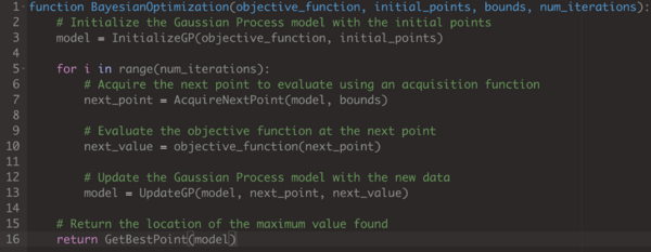
Here, $u$ represents the acquisition function and $D_{1:t-1}=\{(x_{1},y_{1}),...,(x_{t-1},y_{t-1})\}$ are the $t-1$ the observations (where $x_{i}$ is the input variable and $y$ is the outcome) sampled so far from $f$. The pseudo code for BO process goes as follows:

Pesudo Code for Bayesian Optimization process

Here, objective_function is the function to be optimized, initial_points are some of the initial observations from the objective function $f$, bounds are the constraints on the parameters (it specifically represents the range of the variables to optimize), and num_iterations is the number of iterations to run the optimization for. The InitializeGP function initializes the Gaussian Process model with the initial points (it would use a default Gaussian Prioir if the initial_points is null), the AcquireNextPoint function selects the next point to evaluate using an acquisition function, UpdateGP updates the model with the new data, and GetBestPoint returns the location of the maximum value found.

EI is the most widely used acquisition function. Formally EI is defined as

$EI(x)={\begin{cases}(\mu (x)-f(x^{+})-\xi )\varphi (Z)+\sigma (x)\phi (Z)&{\text{if }}\sigma (x)>0\\0&{\text{if }}\sigma (x)=0\end{cases}}$

$Z={\begin{cases}({\frac {\mu (x)-f(x^{+})-\xi }{\sigma (x)}}&{\text{if }}\sigma (x)>0\\0&{\text{if }}\sigma (x)=0\end{cases}}$

Here $\mu (x)$ and $\sigma (x)$ is the mean and standard deviation predicted at $X=x$. $\varphi (Z)$ and $\phi (Z)$ are the CDF and PDF of the standard normal distribution, respectively. The first term in $(\mu (x)-f(x^{+})-\xi )\varphi (Z)+\sigma (x)\phi (Z)$ represents exploitation while the second term quantifies exploration. The first term calculates the potential improvement of the function value at the input point $x$ relative to the current best observed value. This aspect of the acquisition function prioritizes exploitation by identifying the input point with the highest potential to improve upon the current best solution. In other words, it seeks to exploit the current best solution by selecting the input point that has the greatest potential to make a significant improvement. The second term in the EI represents exploration because it is a function of GPs standard deviation or uncertainity ($\sigma (x)$). BO will prefer a point $x$ to explore if GP has high uncertainity at $x$.

Here the constant $\xi$ is used as a hyperparameter to balance the trade off between exploration and exploitation. A pseudo code of the acquisition function is given as follows:

The expected improvement (EI) criterion is based on the intuition of selecting the next input point that has the greatest potential to enhance the current best observed value of the objective function. This approach aims to strike a balance between exploration and exploitation by prioritizing unexplored regions of the input space that have the potential for a substantial improvement over the current best solution.

Pseudo code for Expected Improvement (EI)

End-to-end Example

In order to illustrate an example I used some parts of code from the colab notebook available publicly.

Lets consider an objective function in the following form:

A sample sin(.) based objective function to optimize

For random values of $X$ and $noise=0.2$, the plot of the noisy objective function looks something like this:

Noisy objective function plot

The above noisy objective plot represents the ground truth knowledge about the objective function $f(x)$ to optimize. Here the noise free objective is the set of observations when noise is set to 0.

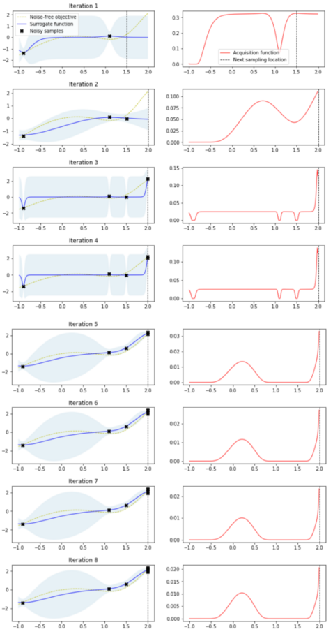
Once the BO process starts, in the first iteration, when the optimizer has no previous observation data, the optimizer randomly picks a point from the search space and evaluates $f$. Based on the generated observational data from the evaluation, the BO updates its GP model (as shown in the pseudo code of BO process). From the second iteration onwards, the AcquireNextPoint function randomly generates hundreds of values of $X$ and computes the acquisition value (using the expected_improvement) for each $X$. Further it picks the $X$ having maximum acquisition value to explore next.

For next 8 iterations, a graphical representation with two plots is generated (for individual iteration). The plot on the left displays the true objective function, the surrogate model represented by the GP posterior predictive mean, the 95% confidence interval of the mean, and the previously gathered noisy samples from the objective function. The right plot illustrates the acquisition function. A vertical dotted line appears in both plots, indicating the selected sample point for the next iteration, which is determined by the highest point of the acquisition function.

BO Iterations representing the search in the search-space

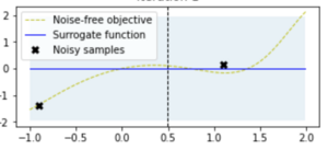
The BO exploration and exploitation starts with a prior which is represented in the approximation plots (surrogate function). Here the initial prior is a straight line represented as follows:

Default prior as a straight line (surrogate function)

With the prior (represented by a straight line at $f(x)=0$), the BO starts exploration. At this point the GP model does not have any knowledge about the function to optimize hence it has same uncertainity (blue marked region around the surrogate function line) at all the regions of $x$. However, we bootstrap the surrogate model with an initial knowledge about only two noisy samples and hence it trains the GP model with these two observations from where the first iteration starts. Here the prior (for the surrogate function) is set when we first initialize the GP model. We can bootstrap it with a specific mean and standard deviation, where it assumes a default mean at 0 and standard deviation as 1.

In every iteration, BO picks the value of $x$ to explore next based on the region in the acquisition plot which has maximum value. It then evaluates the function $f$ at $x$ and updates the GP with the new observation. The marked blue region in the approximation plot (plots in the left) represents the uncertainity of the GP model. Also it is interesting to see the sampled points to explore next. In particular, the sampling strategies in BO often prioritize exploration over exploitation by selecting points that fall within regions of high uncertainty, rather than simply maximizing the surrogate function values (exploitation). This approach aims to balance the search between discovering new promising regions of the input space and refining the current best solution by selecting input points that have the potential to significantly improve the objective function.

Conclusion

Bayesian optimization is an effective method for optimizing functions that are expensive or difficult to evaluate. This technique combines a probabilistic model of the objective function with an acquisition function to efficiently explore and exploit the input space. By iteratively selecting input points based on the expected improvement of the surrogate function, Bayesian optimization can converge to the optimal solution with a small number of function evaluations.

To Add

Put links and content here to be added. This does not need to be organized, and will not be graded as part of the page. If you find something that might be useful for a page, feel free to put it here.