Template:ASTR508/The Evolution of a Low-Mass Star

The Evolution of a Low-Mass Star

Reading Assignment

Chapter 11 of Stellar-Astrophysics Notes

Homology

Often in stellar structure one process dominates in a particular region of the star or possibly in the entire star. Furthermore, the form of the equations like the ones above may be multiplicative in nature which can allow us to find scaling relations between the star's mass and its other properties. Let us write

$q={\frac {M_{r}}{M}}$

and write the various other quantities as a function of $q$ scaled by the total mass to various powers. We have

$P=M^{\alpha _{p}}{\bar {p}}(q),L=M^{\alpha _{L}}{\bar {l}}(q),r=M^{\alpha _{r}}{\bar {r}}(q),T=M^{\alpha _{T}}{\bar {t}}(q).$

To make further progress let's write all of the stellar structure equations in terms of the enclosed mass

${\frac {dP}{dM_{r}}}=-{\frac {GM_{r}}{4\pi r^{4}}},{\frac {dr}{dM_{r}}}={\frac {1}{4\pi r^{2}\rho }},{\frac {dL_{r}}{dM_{r}}}=\epsilon -\epsilon _{\nu },{\frac {dT}{dM_{r}}}=-{\frac {3\kappa L_{r}}{256\pi ^{2}r^{4}\sigma T^{3}}}$

and substitute the scaling relations

$M^{\alpha _{p}-1}{\bar {p}}'=-{\frac {GqM}{4\pi M^{4\alpha _{r}}{\bar {r}}^{4}}},{\bar {p}}'=-{\frac {Gq}{4\pi {\bar {r}}^{4}}}M^{2-4\alpha _{r}-\alpha _{p}}.$

This yields a relationship between the various exponents, $2-4\alpha _{r}-\alpha _{p}=0$. Let's look at the next equation. This has $\rho$ on the right-hand side, so we need a relationship between $\rho$ and the other quantities. This is called the equation of state

$P(\rho ,T)=P_{0}\rho ^{\beta _{\rho }}T^{\beta _{T}}.$

For an ideal gas $\beta _{\rho }=\beta _{T}=1$. For a degenerate gas (non-relativistic), $\beta _{\rho }={\frac {5}{3}}$ and $\beta _{T}=0$. For a neutron star stuff $\beta _{\rho }=2$ and $\beta _{T}=0$. We will leave this quantities open for now, so we have

$\rho =\left[{\frac {P}{P_{0}T^{\beta _{T}}}}\right]^{1/\beta _{\rho }}=P_{0}^{-1/\beta _{\rho }}M^{\alpha _{p}/\beta _{\rho }}{\bar {p}}^{1/\beta _{\rho }}M^{-\alpha _{T}\beta _{T}/\beta _{\rho }}{\bar {t}}^{-\beta _{T}/\beta _{\rho }}$

$M^{\alpha _{r}-1}{\bar {r}}'={\frac {1}{4\pi \rho M^{2\alpha _{r}}{\bar {r}}^{2}}}={\frac {1}{4\pi {\bar {r}}^{2}}}M^{-2\alpha _{r}}P_{0}^{1/\beta _{\rho }}M^{-\alpha _{p}/\beta _{\rho }}{\bar {p}}^{-1/\beta _{\rho }}M^{\alpha _{T}\beta _{T}/\beta _{\rho }}{\bar {t}}^{\beta _{T}/\beta _{\rho }}$

so

$\alpha _{r}-1=-2\alpha _{r}-{\frac {\alpha _{p}}{\beta _{\rho }}}+{\frac {\alpha _{T}\beta _{T}}{\beta _{\rho }}}.$

Temperature-Independent Equations of State

If the equation of state does not depend on temperature ($\beta _{T}=0$), these two equations are sufficient to figure things out. The energy generation and the energy transport equations are important to see how the star shines but not for the structure of the star. We have

$3\alpha _{r}-1=-{\frac {\alpha _{p}}{\beta _{\rho }}},2-4\alpha _{r}-\alpha _{p}=0$

so

$\alpha _{p}={\frac {2\beta _{\rho }}{3\beta _{\rho }-4}},\alpha _{r}={\frac {\beta _{\rho }-2}{3\beta _{\rho }-4}}$

We can see a couple of interesting things immediately. First for $\beta _{\rho }>2$ stars get bigger as they get more massive and for $\beta _{\rho }<2$ more massive stars are smaller in radius. Of course, these equations can apply to any self-gravitating object that ends up spherical and where energy generation doesn't play a role in the structure. For example the radii of objects more massive than Jupiter up until nuclear burning starts are all quite similar, so $\beta \approx 2$ for these objects. This is thought to be also the case for neutron stars.

The second interesting value of $\beta _{r}$ is ${\frac {4}{3}}$ for which both $\alpha _{r}$ and $\alpha _{p}$ diverge. This indicates that the mass for $\beta _{\rho }={\frac {4}{3}}$ has a fixed value that doesn't depend on the central pressure or the radius of the star, rather it depends on the constant $P_{0}$ that we defined earlier. Relativistic degenerate electrons have $\beta _{\rho }\approx {\frac {4}{3}}$ yielding the Chandrasekhar limit for white dwarfs. On the other hand, convective regions also have $\beta _{\rho }\approx {\frac {4}{3}}$ so the mass of such a region does not depend on its radius but rather on the specific entropy of the fluid which in this case sets $P_{0}$ --- this limit applies for low-mass stars which are fully convective.

The $\beta _{\rho }\approx {\frac {4}{3}}$ limit can also be used to understand the most massive stars where radiation pressure dominates. Let us suppose that the pressure due to material is some fraction $\beta$ of the total pressure, so

$R\rho T+aT^{4}=P_{\mathrm {total} }={\frac {1}{\beta }}R\rho T$ and $R\rho T={\frac {\beta }{1-\beta }}aT^{4}$

so

$\rho ={\frac {aT^{3}\beta }{R(1-\beta )}}~{\textrm {or}}~T^{3}={\frac {R\rho }{a}}{\frac {1-\beta }{\beta }}$

and the total pressure is

$P={\frac {1}{1-\beta }}aT^{4}={\frac {1}{1-\beta }}a\left({\frac {R\rho }{a}}{\frac {1-\beta }{\beta }}\right)^{4/3}$

and $\beta _{\rho }={\frac {4}{3}}$.

We know that the pressure within a star must increase as the mass increases, so we find that as the star gets more massive $\beta \rightarrow 0$ and radiation pressure dominates more and more.

A third interesting limit is a constant density object like a rocky planet (approximately). Here $\beta _{\rho }\rightarrow \infty$ so we have $\alpha _{p}={\frac {2}{3}},\alpha _{r}={\frac {1}{3}}$ and the radius increases as the cube root of the mass (which makes sense) and the pressure increases as mass to the two-thirds power.

Temperature-Dependent Equations of State

To make further progress (and to have stars that shine) we will have to tackle the other equations of stellar structure. And these require us to define some more constitutive relations. We have the energy generation equation

${\frac {dL_{r}}{dM_{r}}}=\epsilon -\epsilon _{\nu }=\epsilon _{0}\rho ^{\gamma _{\rho }}T^{\gamma _{T}}=\epsilon _{0}P^{\gamma _{\rho }/\beta _{\rho }}T^{\gamma _{T}-\beta _{r}ho\gamma _{\rho }/\beta _{T}}$

where we have used the equation of state to eliminate the density from the equation.

For many energy generation processes $\gamma _{T}$ is large and $\gamma _{\rho }\approx 1$.

$M^{\alpha _{L}-1}{\bar {l}}'=\epsilon _{P}M^{\alpha _{P}\gamma _{\rho }/\beta _{\rho }}{\bar {p}}^{\gamma _{r}ho/\beta _{\rho }}M^{\alpha _{T}\left(\gamma _{T}-\beta _{\rho }\gamma _{\rho }/\beta _{T}\right)}{\bar {t}}^{\gamma _{T}-\beta _{\rho }\gamma _{\rho }/\beta _{T}}$

so

$\alpha _{L}-1={\frac {\alpha _{P}\gamma _{\rho }}{\beta _{\rho }}}+\alpha _{T}\left(\gamma _{T}-{\frac {\beta _{\rho }\gamma _{\rho }}{\beta _{T}}}\right)$

We get the following relationships between the exponent of $M$:

$\alpha _{P}-1=1-4\alpha _{r}$

$\alpha _{r}-1=-2{\frac {\alpha _{r}\beta _{\rho }+\alpha _{P}-\beta _{T}\alpha _{T}}{\beta _{\rho }}}$

$\alpha _{L}-1={\frac {\gamma _{\rho }\alpha _{P}-\gamma _{\rho }\beta _{T}\alpha _{T}+\gamma _{T}\alpha _{T}\beta _{\rho }}{\beta _{\rho }}}$

$\alpha _{T}-1={\frac {\delta _{r}ho\alpha _{P}-\delta _{\rho }\beta _{T}\alpha _{T}+\delta _{T}\alpha _{T}\beta _{\rho }+\alpha _{L}\beta _{\rho }-4\alpha _{r}\beta _{\rho }-3\alpha _{T}\beta _{\rho }}{\beta _{\rho }}}$

and the solutions

$\alpha _{L}={\frac {-16-\gamma _{T}\beta _{\rho }-2\gamma _{\rho }\delta _{T}+2\gamma _{T}\delta _{\rho }-3\delta _{T}\beta _{\rho }+8\gamma _{\rho }+\gamma _{\rho }\beta _{T}+4\gamma _{T}+12\beta _{\rho }+4\beta _{T}+3\delta _{\rho }\beta _{T}+4\delta _{T}}{D}}$

$\alpha _{P}=2{\frac {4\beta _{\rho }-\gamma _{T}\beta _{\rho }-\delta _{T}\beta _{\rho }+\gamma _{\rho }\beta _{T}+\delta _{\rho }\beta _{T}}{D}}$

$\alpha _{r}={\frac {4\beta _{\rho }-8-\gamma _{T}\beta _{\rho }-\delta _{T}\beta _{\rho }+2\beta _{T}+\gamma _{\rho }\beta _{T}+2\delta _{T}+\delta _{\rho }\beta _{T}+2\gamma _{T}}{D}}$

$\alpha _{T}=2{\frac {\delta _{\rho }+\gamma _{\rho }+\beta _{\rho }}{D}}$

where

$D=12\beta _{\rho }-3\delta _{T}\beta _{\rho }+4\beta _{T}-16+3\delta _{\rho }\beta _{T}+4\delta _{T}-3\gamma _{T}\beta _{\rho }+3\gamma _{\rho }\beta _{T}+4\gamma _{T}$

These are completely general and completely useless. Let's look at thermal pressure from ions ($\beta _{\rho }=\beta _{T}=1$) and free-free opacity ($\delta _{\rho }=1$, $\delta _{T}=-7/2$). Furthermore let's focus on hydrogen burning with $\gamma _{\rho }=1$. We are left with

$\alpha _{L}={\frac {31+10\gamma _{T}}{5+2\gamma _{T}}},\alpha _{P}={\frac {38-4\gamma _{T}}{5+2\gamma _{T}}},\alpha _{r}={\frac {-7+2\gamma _{T}}{5+2\gamma _{T}}},\alpha _{T}={\frac {12}{5+2\gamma _{T}}}$

For nuclear energy generation processes $\gamma _{T}$ is large so if we take the limit of $\gamma _{T}\rightarrow \infty$ we have

$\alpha _{L}=5,\alpha _{P}=-2,\alpha _{r}=1,\alpha _{T}=0.$

As the mass increases the typical density decreases, so eventually free-free opacity is less than electron scattering opacity with $\delta _{T}=\delta _{\rho }=0$ and

$\alpha _{L}=3,\alpha _{P}=-2,\alpha _{r}=1,\alpha _{T}=0.$

The luminosity dependence on mass is somewhat more relaxed. Finally at the highest mass stars, the pressure is also dominated by the radiation so additionally we have $\beta _{\rho }=0$ and $\beta _{T}=4$ and

$\alpha _{L}=1,\alpha _{P}=0,\alpha _{r}={\frac {1}{2}},\alpha _{T}=0.$

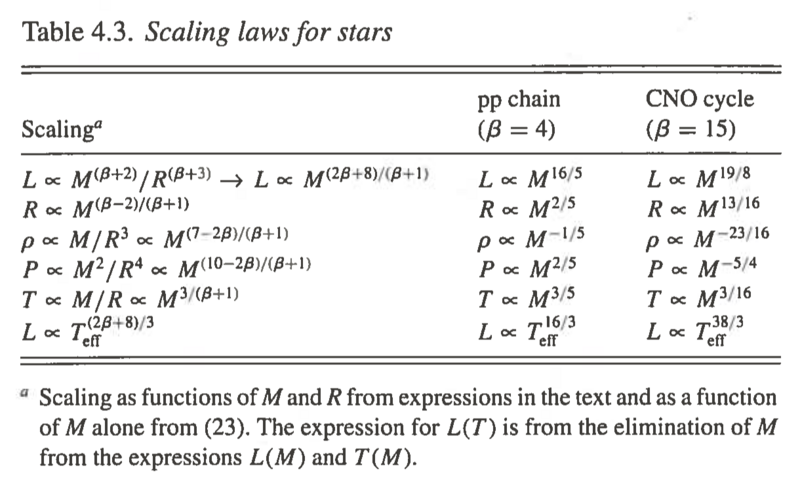
These relationships reflect the observed mass-luminosity for stars more massive than about half of the mass of the Sun. Less massive stars are fully convective and our analysis did not include convection at all so it cannot apply to these stars.

MESA

MESA Inlists:

• 1M_pre_ms_to_wd (long test)
• solar_calibration
• solar

Stellar Structure of Low-Mass Stars

Assignment

1. Using sample_zams as a starting point, generate a CMD in MV vs B-V for a solar metallicity ZAMS and for the metallicity of 47 Tuc (create_zams). If you assume that stars stay the same colour and luminosity on the MS (not strictly true), what does the CMD look like at an age of 10 Myr, 100 Myr, 1 Gyr and 10 Gyr? Using your solar metallcity ZAMS at 100 Myr figure out the distance to the Pleiades and at 10 Gyr for 47 Tuc. You will have to edit the specification file. Use the value of log(tnuc) to estimate which stars are alive after a given time. That is, for 1 Gyr only plot stars with log(tnuc)>9.

For the 47 Tuc model with (create_zams) you will have to remove the line from run_star_extras.f that gets it to stop (look in the docs directory for a hint) and put a control in run_star.extras.f to get it to stop at the end of H-burning, say when the central hydrogen fraction is less than one percent. You can use the star pointer variable: s % center_h1. Make it like the code that you just deleted. The routines create_zams and sample_zams do not make files in the LOG directory, so you will use the final console output to get the data that you need.

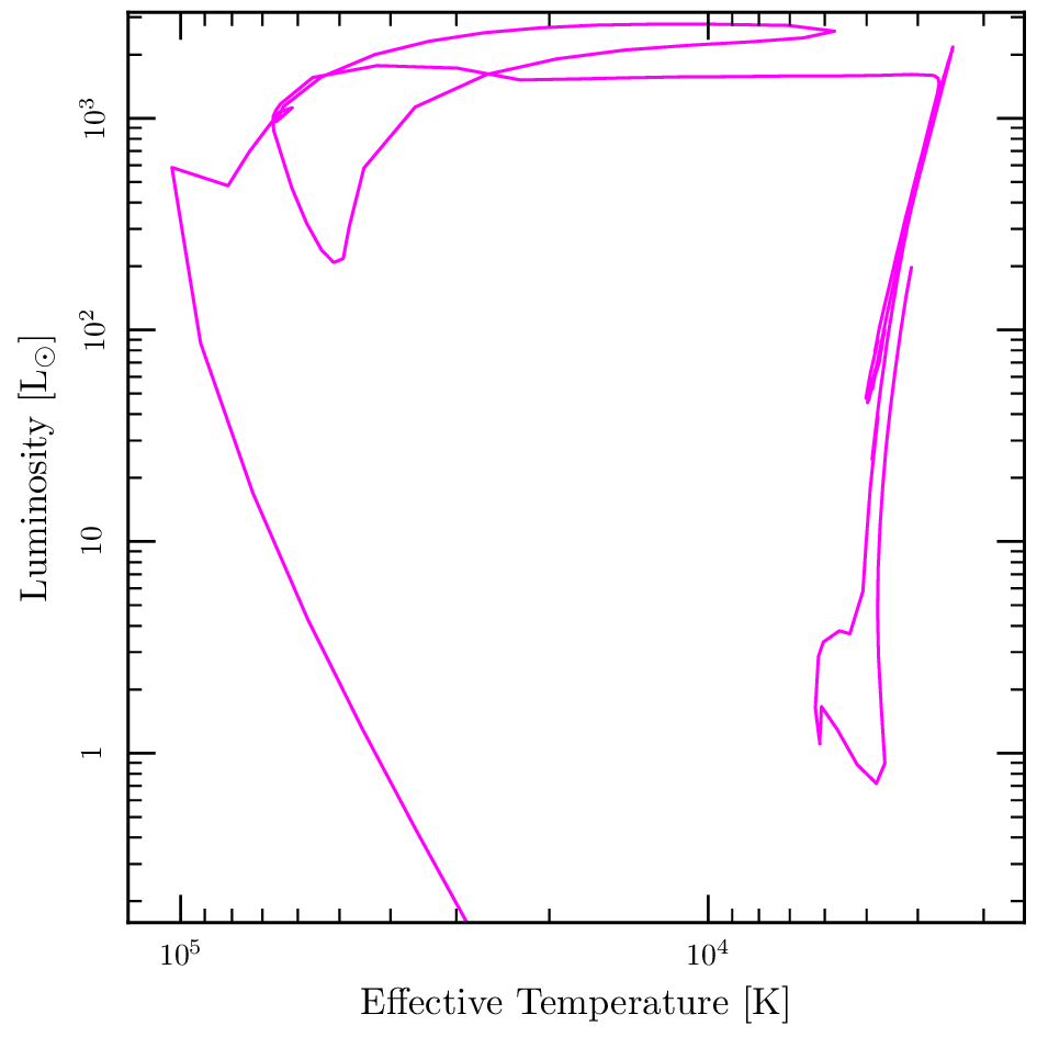
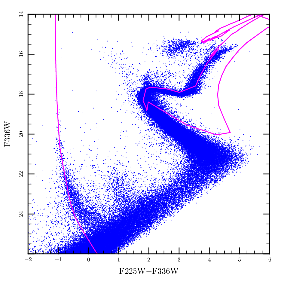
1. Generate a CMD for a solar mass star through its entire lifetime (here both L vs Teff and MV vs B-V). Divide the star's history into various stages by looking at the external observables as a function of time. What is going on inside the star during each of these stages? Start with the 1M_pre_ms_to_wd inlist.

You will find the table below useful to convert luminosity and effective temperature to colour.

# SpTyp  MV   BC   MBol   B-V   L/Lsun    Teff  Mass
#  1     2    3     4      5      6        7      8 
  M6  16.5   4.3 12.20  1.7  1.0568e-03   2600  0.17
  M4  12.7   2.7 10.00  1.6  8.0168e-03   3200  0.25
  M2  11.2   1.7  9.50  1.5  1.2706e-02   3400  0.3
  M0   8.9   1.2  7.70  1.41 6.6681e-02   3800  0.35
  K7   8.3   1.0  7.30  1.32 9.6383e-02   4000  0.47
  K5   7.5   0.6  6.90  1.08 1.3932e-01   4350  0.69
  K0   5.9   0.4  5.50  0.84 5.0582e-01   5250  0.78
  G5  4.93   0.2  4.73  0.69 1.0280e+00   5700  0.93
 Sun  4.83  0.07  4.76  0.65 1.0000e+00   5780  1
  G0   4.2   0.2  4.00  0.59 2.0137e+00   6000  1.10
  F5   3.3   0.1  3.20  0.41 4.2073e+00   6500  1.3
  F0   2.4   0.1  2.30  0.32 9.6383e+00   7300  1.7
  A5   1.8   0.1  1.70  0.19 1.6749e+01   7800  2.1
  A0   0.8   0.3  0.50  0.0  5.0582e+01   9400  3.2
  B8 -0.25   0.8 -1.05 -0.11 2.1086e+02  11600  4
  B6  -1.0   1.2 -2.20 -0.14 6.0814e+02  14000  5
  B3  -1.4   1.6 -3.00 -0.18 1.2706e+03  18750  11
  B0  -3.7   3.0 -6.70 -0.30 3.8371e+04  30500  18
  O8  -4.3   3.3 -7.60 -0.321 8.7902e+04  35000  20
  O5  -5.2   3.8 -9.00 -0.322 3.1915e+05  41000  35
  O3  -5.8   4.0 -9.80 -0.323 6.6681e+05  44500  40

To log out from your computer but still have your job run, you will need to disown the job. Here is how. Type "jobs" at the prompt. Find the job in question, and type "disown %1" if it is job number 1. If you type "jobs" again you should find that the job is no longer on the list. If you run "top", you will see the job on the top of the list and you can kill it if you want by typing in the job number.

We have developed a more sophisticated tool to convert the MESA output files to the observable fluxes. It is called paintisochrone.py You can download it at

gcwd.tar.gz

with instructions and lots of ancillary files so that you can try it out.

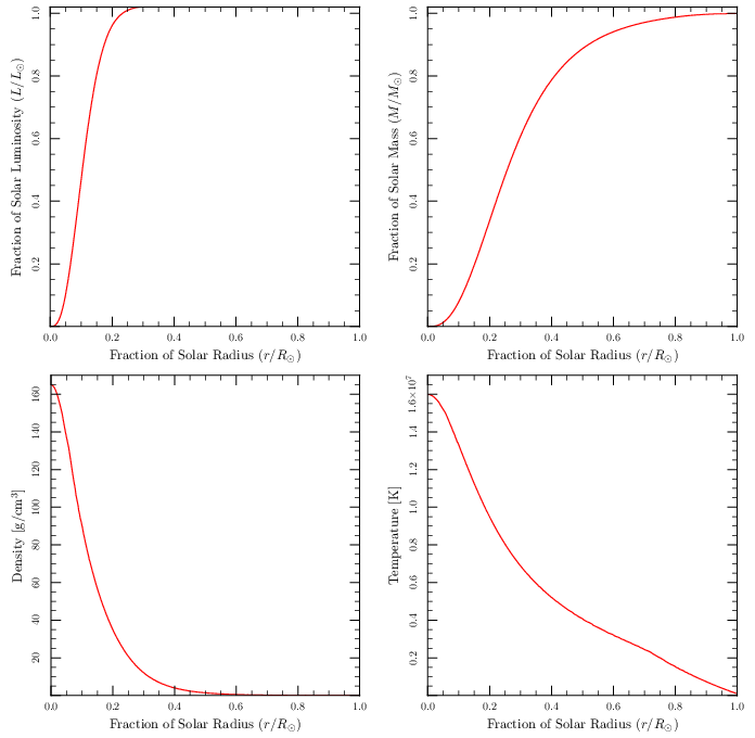
Let's build upon the solar models that you performed in Week 2. Run the a one-solar-mass model using 1M_pre_ms_to_wd. Idenify the various regions on the H-R diagram for the main sequence, giant branch, horizontal branch and asymptotic giant branch and plot the profiles of density, temperature, energy generation as a function of radius for each stage. Also plot temperature against density on a log-log plot to identify the convective and radiative regions.

Repeat the analysis for a 0.3 solar-mass star and a 3 solar-mass star.