Soil Texture - Hydrometer Method

Introduction

The hydrometer method of determining soil texture is a more involved sedimentation method, and used for soils finer than 2 mm for precise quantitative estimates. Because the coarse and very coarse sand settles out too quickly for accurate determination by sedimentation, a combination of sieving (down to 0.5 mm) and sedimentation is sometimes used.

The two most common applications of sedimentation are the pipette method and the hydrometer method. This page covers the hydrometer method. The amounts of silt and clay (+/- sand) are usually determined by a sedimentation procedure, which uses a basic principle of sedimentation called "Stoke’s Law": because soil particles are denser than water, they tend to sink, settling at a velocity that is proportional to their size. In other words, the bigger the particle, the faster it will fall. Data is collected with a hydrometer often called a Bouyoucos hydrometer after the scientist who invented it. The hydrometer indicates the density of the suspension at its centre of buoyancy. If the suspension is very dense, the hydrometer does not sink very much. On the contrary, if the suspension density is low the hydrometer will sink deeper. The density of the suspension depends on the amount of soil particles still in suspension so the hydrometer provides a measure of how much soil is still suspended at any given time.

Figure 1. Hydrometer lab set up

Sedimentation Theory - Stoke's Law

Stoke’s Law states that the speed or velocity (V) of a particle falling through a fluid is directly proportional to the gravitational force g, the difference between the density of the particle (ρs) and the density of the fluid (ρL), and the square of the effective particle diameter (D squared). The settling velocity is inversely proportional to the viscosity or “thickness” of the fluid (η). Since velocity equals distance Z divided by time t Stoke’s Law can be written as:

Stoke's Law

Note: Stoke’s Law is based on certain simplifying assumptions:

1. All soil particles have the same density

2. Particles are spherical, smooth, and rigid

3. The suspension is sufficiently dilute such that particles do not interact with each other or the container

4. There is no Brownian motion of fluid molecules

5. There is no turbulence, i.e. fluid flow around particles is laminar

The distance Z represents depth of fall by the particle in the time t. The depth Z is called effective depth of measurement. The diameter of the particle (D) corresponding to a known depth Z is calculated by rearranging the previous equation:

Additional details

Data are collected with a hydrometer often called a Bouyoucos hydrometer after the scientist who invented it.

The hydrometer indicates the density of the suspension at its center of buoyancy. If the suspension is very dense, the hydrometer does not sink very much. On the contrary if the suspension density is low the hydrometer will sink deeper. The density of the suspension depends on the amount of soil particles still in suspension so the hydrometer provides a measure of how much soil is still suspended at any given time.

Materials

1. Soil samples
   

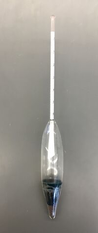
   Figure 2. LFS Hydrometer
2. Hydrogen peroxide (H₂O₂)
3. Sodium Hexametaphosphate (${\ce {Na4P2O7}}$)
4. 1000ml graduated cylinders
5. Milkshake blenders
6. Amyl alcohol
7. Watch Glasses
8. Hydrometer (Figure 1)

Procedure

1. Sample Preparation

As the first step, organic matter that serves as a cementing agent has to be destroyed. For this we usually use hydrogen peroxide.

**Procedure: Removing Organic Matter**

1. Record the weight of a clean, dried 600ml beaker. Add 40.00 g of soil
2. Make up to the 300 ml mark with distilled water and stir
3. Carefully, to avoid excessive foaming, add hydrogen peroxide (H₂O₂) in 10-20 ml increments until the reaction slows, indicating completion. If too much foaming occurs, add a few drops of amyl alcohol.
4. Leave at room temperature for 2 days. A Watch Glass should be placed over the beakers to prevent clay from spattering out. Wash Watch Glasses into beakers.
5. Heat on a hot plate to about 80°C until excess H₂O₂ is removed (at least 4-5 hours). Check by the addition of a small amount of H₂O₂ that all the organic matter has been destroyed (Figure 3.)
6. Removed from heat.
7. Oven-dry at 105°C for 24 hours. Cool and record the final weight of the beaker plus sample.
   

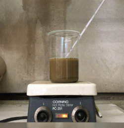
   Figure 3. Step #5 of sample preparation

Following the procedure above, all the soil particles have to be separated from each other (i.e. dispersed) in order for the following procedure to work. Dispersant solution (e.g. sodium hexametaphosphate) is added to 40 g of soil and the soil is mechanically stirred on a shaker. Dispersant solution separates all the clay particles and breaks apart the soil aggregates.

Next the suspension (a mixture of soil particles and liquid) is transferred into a 1000-mL sedimentation cylinder and distilled water is added until the volume reaches 1000 mL. A blank sample is also prepared by pouring 50 mL of the dispersant solution and 950 mL of distilled water into a sedimentation cylinder. Cylinders and their contents should be brought to a known, constant temperature before proceeding with sedimentation analysis.

2. Data Collection

**Take sample readings**

1. Mix the suspension thoroughly using a rod with a disk on the end. Lift it gently up and down the cylinder.
2. Lift the rod out and note the time
   

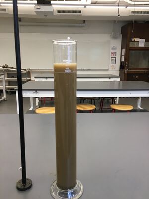
   Figure 4. Step # 1 of taking sample readings.
3. After approximately 10 seconds slowly insert the hydrometer into the cylinder. Use your finger to steady the hydrometer
4. Record readings at the base of the meniscus at 30, 50, 70, and 90 seconds after lifting the rod out of the suspension
5. Repeat all previous steps 3 times and calculate an average reading for each time
6. Record the average reading on the DATA COLLECTION SHEET FOR HYDROMETER METHOD

Then,

**Take a blank reading**

1. Insert your hydrometer into the blank cylinder and steady it. The blank cylinder contains distilled water.
2. Once the hydrometer is steady record the blank reading. It should not vary with time since there are no particles settling.

Data Collection Sheets

Here is a potential set of data collection sheets that can be referenced from the calculation beneath.

A potential set of data collection sheets.

Figure 5. Blank hydrometer example

3. Calculation

1) For each reading (R) calculate the effective depth of measurement (Z) by using the equation:

$Z=(-0.00164R)+0.163$[m]

This equation is base on dimensions of a standard ASTM 152H soil hydrometer and a standard sedimentation cylinder. The effective depth of measurement is the depth of the hydrometer bulb below the initial level, and not the depth below the surface during measurement, because fluid is displaced by the hydrometer.

Then, calculate particle diameter (D) using Stoke's Law:

$D=1000{\sqrt {\frac {YZ}{t}}}$ [mm]

The factor of 1000 converts to mm from the units of m.

2) For each measurement calculate the concentration C of particles remaining in suspension:

$C=R-R_{1}$ [g L^-1]

Subtraction of the hydrometer reading for the blank solution (R_L) corrects the R reading for temperature effects on hydrometer buoyancy and for any error in hydrometer zero calibration.

Then calculate the mass percentage of the soil sample smaller than D (P_D), corresponding to each measurement:

$P_{D}=100C/B$ [%]

B is the mass of soil sample per suspension volume (set to 40 g L^-1 )

3) On semi-logarithmic paper (to be provided during the lab) plot the dependent variable P_D (on the linear y axis) versus the independent variable D (on the logarithmic x axis).

Draw a smooth ‘best fit’ curve using the 7 data points. This curve is known as the particle size distribution curve.

4) For D = 0.05 mm (the sand-silt boundary) and D = 0.002 mm (the silt-clay boundary) find P_D by interpolation on your graph.

5) Determine percent clay, silt and sand as follows:

P_0.002 = percent clay (you get this directly from the graph)

P_0.05 – P_0.002 = percent silt (both P_0.05 and P_0.002 values are obtained from the graph)

100 – P_0.05 = percent sand (P_0.05 value is obtained from the graph)

References

1. Gee, G.W. and Bauder, J.W. 1986. Particle-size analysis. p. 383-411. In A. Klute (ed.) Methods of soil analysis. Part 1. 2nd ed., Agron. Monogr. 9. ASA-SSSA, Madison, WI.
2. Lavkulich, Lesley. 1981. Particle Size Analysis - Hydrometer Method Using Computer Program. In Methods Manual - Pedology Laboratory. p. 129-130. 3rd printing. University of British Columbia, Vancouver, BC.