Graph Neural Networks

Introduction

Graphs are a type of data structure that consist of nodes and edges, and they are commonly found in natural sciences, social sciences, and the web. Unlike images, audio, and language, the underlying data in graphs is non-euclidean, which means it cannot be fully represented in euclidean spaces. This poses a challenge for applying standard deep learning techniques like Convolutional Neural Networks (CNNs) and Recurrent Neural Networks (RNNs) to model such data. In order to address this challenge, researchers have developed a class of deep learning methods known as Graph Neural Networks (GNNs). Bronstein et al. provide an overview of applying deep learning techniques to non-euclidean data like graphs and manifolds. GNNs operate on graphs by propagating information through nodes and edges, enabling them to learn complex relationships and dependencies between nodes. They can be used for a variety of tasks, including node classification, link prediction, and graph classification. In this article, we cover graphs, their structure, GNNs and the math behind GNNs.

Structure of Graphs

First, we need to understand the graph data structure. A graph consists of relations (edges) between entities (nodes). The following features are also commonly present,

1. $V$: Vertex (or node) attributes like node identity, number of neighbours
2. $E$ : Edge (or link) attributes like edge weight
3. $U$ : Global graph attributes like number of nodes, longest path

There are two commonly used data-structures to represent graphs,

1. Adjacency Matrix

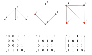
One common way to represent connections in a matrix is using the adjacency matrix. If a graph contains N nodes, the adjacency matrix is an N x N matrix, with $a_{ij}=1$ if node i and node j are connected else $a_{ij}=0$. Therefore, it only consists of 1s and 0s.

Figure 1: Adjacency Matrix Visualized

2. Adjacency Lists

An adjacency list is an efficient way to store sparse matrices (number of edges << $n_{nodes}^{2}$). It is basically a list storing all the edges in the graph. So for instance, the Adjacency list for the left most graph in Figure 1, would be,

[[1, 4], [2, 4], [3, 4]]. You can see how instead of having to store 16 numbers for the 16 possible edges, we only store the edges.

Figure 2 : Zach's Karate Club is a popular example in this domain with individuals (as nodes) in this club follow one of their two leaders. Predicting which leader (node feature) each individual (node) supports would be an example of node-level prediction.

Modelling Tasks on Graphs

Let's look at three tasks for which GNNs are commonly used,

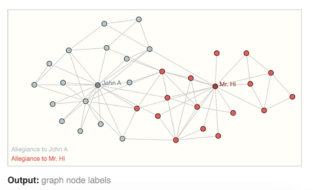
1. Node-Level Prediction: These are concerned with predicting the role/properties of each node within a graph. For instance, figure 2 is a commonly used example.
2. Graph-Level Prediction: These are concerned with predicting the property of the entire graph. For instance, predicting molecular properties like potential energy.
3. Edge-Level Prediction: These are concerned with predicting the presence/property of edges in a graph. For instance, predicting relations between subjects and objects in a knowledge graph.

Motivation for GNNs

Consider the task of predicting a molecular property given atom features. Suppose a molecule has N atoms and each atom/node has 2 features. In that case, the input feature matrix will be an N x 2 matrix. However, there is an issue when using conventional machine learning techniques. If I change the order of the nodes, a neural network will produce a distinct result. Standard neural networks do not have permutation-invariance, which means they can't maintain the same output when the order of nodes is altered. Since the graph's structure has no inherent order, changing the node's sequence should not impact a neural network's output.

To tackle this issue, Graph Neural Networks are designed keeping the permutation-invariance property in mind.

Graph Neural Networks

We will describe the working of these networks before going into mathematical details. A GNN generally consists of the following layers,

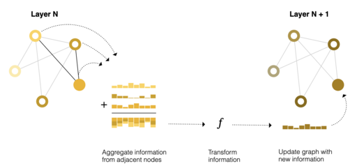
• Message Passing Layers: Update node by aggregating messages from neighbours
• Pooling Layer: Pool node embeddings to get a single graph level embedding

The embeddings of nodes, edges, and sometimes even entire graphs are learned during the training process, depending on the task at hand. Initially, these embeddings can be established using the properties of nodes, edges, and graphs.

Figure: Message passing Layer

Message Passing Layers

Typically, message passing layers update embeddings for each node $i$ using following three steps,

1. Gather the node and edge embeddings of all the neighbours $j\in {\mathcal {N}}_{i}$ where ${\mathcal {N}}_{i}$ is the set of neighbours of node $i$
2. Aggregate them using a specified function (sum, max, mean, attention, etc).
3. Update the aggregated message using a neural network

Different variants of GNNs have different variations in how the message passing is done but the broad set of steps remain the same.

Pooling Layers

In these layers, the embeddings from the previous message passing layer are utilized and then pooled/aggregated to generate a single representation for the complete graph. These representations can be employed for downstream tasks, such as graph-level predictions. Commonly used pooling schemes are average, mean, sum, max.

How do GNNs guarantee permutation-invariance?

An important aspect of GNNs is permutation-invariance. If we look at the two components of GNNs carefully,

• Message Passing Layers possess permutation-equivariance, as they update the embeddings of nodes based on their neighbors, independent of the node order. Therefore, the network can recognize the same graph structure regardless of the node ordering, which is crucial for graph-based tasks where the node order should not affect the model's predictions.
• Pooling layers have permutation-invariance, which means that the output remains the same regardless of the order of the input. This is because pooling operations, such as max or average pooling, are commutative and associative, and do not rely on the ordering of the input elements. Therefore, the pooling layer output remains unchanged even if the order of nodes is permuted in the input graph.

Therefore, combining the two you can see how GNNs handle permutations to node order.

Popular Variants of Graph Neural Networks

There are various popular graph neural networks in literature. We look at two important variants,

1. Graph Convolutional Networks (GCN)
2. Graph Attention Networks (GAT)

In the equations shown below, $h_{v}^{(l)}$ represents node embeddings of node $v$ at the $l^{th}$ message passing layer and ${\mathcal {N}}_{v}$ represents neighbours of node $v$. Initially, they are set to node features and then are iteratively learned.

Graph Convolutional Networks (GCNs)

Intuition: In each GCN layer, we average the embeddings of the neighbours, transform it with linear weights and a non-linearity. By doing so we update the node embedding with the information of its neighbours in each GCN layer.

Message passing layers of GCNs perform the following,

$$h_{v}^{(k)}=f^{(k)}{\bigg (}W^{(k)}\cdot {\frac {\sum _{u\in {\mathcal {N}}(v)}h_{u}^{(k-1)}}{|{\mathcal {N}}(v)|}}+B^{(k)}\cdot h_{v}^{(k-1)}{\bigg )},$$

1. For a node $v$ with embedding $h_{v}^{(k-1)}$, gather the embeddings of neighbouring nodes ($h_{u}^{(k-1)}\mid u\in {\mathcal {N}}(v)$). Sum them and normalize it by the node degree (number of neighbours)
2. Transform the normalized embedding value (${\frac {\sum _{u\in {\mathcal {N}}(v)}h_{u}^{(k-1)}}{|{\mathcal {N}}(v)|}}$) with a weight matrix $W^{(k)}$
3. Transform $h_{v}^{(k-1)}$ using $B^{(k)}$
4. Transform the sum of step 2 and 3 with $f^{(k)}$(like an activation function) to get the new embedding for node $v$

where $W^{(k)}$, $B^{(k)},f^{(k)}$have potential learnable parameters.

For getting graph level embeddings, a permutation-invariant readout layer is used to gather node level embeddings from the last message passing layer $L$ to get a graph level embedding $h_{G}$,

$$h_{G}={\text{READOUT}}(h_{v}^{(L)}\mid v\in G))$$

Graph Attention Networks (GATs)

Intuition: In each GAT layer, instead of equally weighting all neighbour messages like GCNs, we use the attention weights derived using the neighbour and node embeddings. By doing so, we can attend to important messages from neighbours.

GATs use attention weights to aggregate messages from neighbours. The message passing equation for the $k$th layer performs the following steps,

$${\begin{aligned}h_{v}^{(k)}&=f^{(k)}{\bigg (}W^{(k)}\cdot {\bigg [}\sum _{u\in {\mathcal {N}}(v)}\alpha _{vu}^{(k-1)}h_{u}^{(k-1)}+\alpha _{vv}^{(k-1)}h_{v}^{(k-1)}{\bigg ]}{\bigg )}\\\alpha _{vu}^{(k-1)}&={\frac {A^{(k-1)}(h_{v}^{(k-1)},h_{u}^{(k-1)})}{\sum _{w\in {\mathcal {N}}_{v}}A^{(k-1)}(h_{v}^{(k-1)},h_{w}^{(k-1)})}},\end{aligned}}$$

1. For a node $v$ with embedding $h_{v}^{(k-1)}$, gather the embeddings of neighbouring nodes.
2. Perform a weighted sum using attention weights calculated using the usual attention mechanism ($\sum _{u\in {\mathcal {N}}(v)}\alpha _{vu}^{(k-1)}h_{u}^{(k-1)}$).
3. Transform $h_{v}^{(k-1)}$ using self-attention weight $\alpha _{vv}^{(k-1)}$
4. Add the embeddings from step 2 and 3 and transform the dimension with a weight matrix $W^{(k)}$
5. Apply activation $f^{(k)}$ on the output of step 4

where $W^{(k)}$, $f^{(k)},A^{(k-1)}$are learnable parameters. $A^{(k)}$ is using a usual attention mechanism shared across all nodes. We can use a readout layer as described in the previous section to get graph level embeddings.

Problems with Graph Neural Networks

GNNs are useful in building expressive representations and have delivered state of the art performance on various tasks. However, there are certain theoretical challenges associated with graph neural networks because of message passing layers. We have a look at two of those challenges,

Oversmoothing and Overquashing

The phenomenon of oversmoothing happens when repeat aggregations in message passing neural networks cause node features converge. Whereas oversquashing occurs when the receptive field of nodes grows exponentially with each message passing layer. Since node features are fixed-size, aggregating information from a large number of nodes might result in "squashing" of information.

Figure: Message Passing Networks are not able to distinguish between the two graphs

Message Passing Networks are at most 1-WL powerful

Let's look at an example, the figure on the right clearly has two graphs with different structures, but if we apply standard message passing networks like GCN or GAT, it will result in the same graph embedding for the two graphs.

The k-Weisfeiler-Lehman (k-WL) test is a graph isomorphism test that works by iteratively coloring the nodes of a graph based on the multiset of colors of its neighbors and comparing the resulting color sequences. The final histograms of colours are compared and if they are not the same then they are not isomorphic. Standard message passing networks are bounded by 1-WL due to which they are often not able to detect non-isomorphic graphs like shown in the example.

Python Implementations

There have been various packages developed for using GNNs with graph-structured datasets. Some of the commonly used packages are as follows,

1. Deep Graph Library
2. Pytorch Geometric

Follow-up Work

Given the various challenges associated with GNNs, this field has been an active area of research. There has been significant practical and theoretical work done to reduce oversquashing and oversmoothing of GNNs and increase the expressivity of these networks. Some interesting directions are as follows,

• Utilizing the transformer architecture for graphs to allow modelling long-distance node relations
• Improving message passing using multiple aggregators

References

- ↑ Bronstein MM, Bruna J, LeCun Y, Szlam A, Vandergheynst P. Geometric deep learning: going beyond euclidean data. IEEE Signal Processing Magazine. 2017 Jul 11;34(4):18-42.
- ↑ https://distill.pub/2021/gnn-intro/
- ↑ Kipf TN, Welling M. Semi-supervised classification with graph convolutional networks. arXiv preprint arXiv:1609.02907. 2016 Sep 9.
- ↑ Veličković P, Cucurull G, Casanova A, Romero A, Lio P, Bengio Y. Graph attention networks. arXiv preprint arXiv:1710.10903. 2017 Oct 30.
- ↑ Vaswani A, Shazeer N, Parmar N, Uszkoreit J, Jones L, Gomez AN, Kaiser Ł, Polosukhin I. Attention is all you need. Advances in neural information processing systems. 2017;30.
- ↑ Provably expressive graph neural networkshttps://blog.twitter.com/engineering/en_us/topics/insights/2021/provably-expressive-graph-neural-networks
- ↑ Xu K, Hu W, Leskovec J, Jegelka S. How powerful are graph neural networks?. arXiv preprint arXiv:1810.00826. 2018 Oct 1.
- ↑ Kreuzer D, Beaini D, Hamilton W, Létourneau V, Tossou P. Rethinking graph transformers with spectral attention. Advances in Neural Information Processing Systems. 2021 Dec 6;34:21618-29.
- ↑ Corso G, Cavalleri L, Beaini D, Liò P, Veličković P. Principal neighbourhood aggregation for graph nets. Advances in Neural Information Processing Systems. 2020;33:13260-71.