Documentation:Microeconomics Review for FRE Courses
Supply and Demand
Demand
It defines the number of goods or services consumers are willing to purchase at each price. It describes the entire relationship between the price and the quantity demanded.


Review of Key Concepts
- The quantity demanded is the total number of items purchased at each price.
- Law of demand: Other things remain the same, there is an inverse relationship between price and quantity. Hence:
An increase in the price decreases the quantity demanded of that good or service. Similarly, a reduction in the price leads to a rise in the quantity demanded of that good or service
The law of demand results from:
- Substitution Effect: When the price of a good or service increases relative to other similar goods or services, then people look for substitutes for it. This leads to a decrease in the demand for goods or services.
- Income Effect: When the price of a good or service increases and income remains the same, people cannot afford all the items they were used to buying. Then, the quantity demanded of that good or service decreases.

Demand Curve:
It shows the relationship between price and quantity demanded during a particular period. By convention, economist graph the quantity on the horizontal axis and the price on the vertical axis.
Figure 1 shows the hypothetical quantities demanded each month at prices ranging from $2 to $8 per pound. Note that the curve shows that the higher the price, the lower the quantity demanded; therefore, demand curves are downward sloping.
| Watch it! |
|---|
Movements along the demand curve:
- A rise in the price, other things remaining equal, leads to a decrease in the quantity demanded and a movement up along the demand curve. The blue arrow in Figure 2 illustrates this movement.
- Similarly, a fall in the price, other things remaining equal, leads to an increase in the quantity demanded and a movement down along the demand curve. The purple arrow in Figure 2 illustrates this movement.
Change (Shifts) in the demand curve:
Demand changes occur when something influences the consumer’s buying plans other than the price of the good or service. Hence, the quantity of goods or services changes at every possible price. This will lead to a new demand curve.
The consumer buying plans could be affected by changes in income, the prices of related goods, preferences, population or number of consumers, and expectations about the future. The formers are usually referred to as the demand shifters.
- The demand curve shifts to the right when the demand increases. Demand curve 2 in Figure 3 illustrates this shift.
- The demand curve shifts to the left when the demand decreases. Demand curve 3 in Figure 3 illustrates this shift.
| Watch it |
|---|
Supply

It’s defined as the number of goods and services a producer is willing to supply at each price. It describes the entire relationship between the price and quantity the producer supplies. Watch it!

Review of Key Concepts
- The quantity supplied is the total number of items sold at each price.
- Law of Supply: Other things remain the same, there is a positive relationship between price and quantity. Hence:
An increase in the price increases the quantity supplied of that good or service. Similarly, a reduction in the price leads to a fall in quantity supplied of that good or service.
The law of supply results from the marginal cost of production. Producers are willing to supply an item only if they can cover their marginal cost of production.
Supply Curve:

The supply curve shows the relationship between price and quantity supplied during a particular period. By convention, economist graph the quantity on the horizontal axis and the price on the vertical axis. Figure 4 shows the hypothetical quantities supplied each month at prices ranging from $2 to $8 per pound. Note that the curve shows that the higher the price, the higher the quantity supplied. Therefore supply curves are upward sloping.
| Watch it |
|---|
Movements along the supply curve:
- A rise in the price, other things remaining equal, leads to an increase in the quantity supplied and a movement up along the supply curve. The blue arrow in Figure 5 illustrates this movement.
- Similarly, a fall in the price, other things remaining equal, leads to a decrease in the quantity supplied and a movement down along the supply curve. The purple arrow in Figure 5 illustrates this movement.
Change (Shifts) in the supply curve:
A change in supply occurs when something influences the producer’s selling plans other than the price of the good. Hence, the quantity of goods or services changes at every possible price. This will lead to a new supply curve.
The producer selling plans could be affected by changes in the prices of factors of production, the prices of related goods, the number of suppliers, technology advancements, returns from alternative activities, natural events, and expectations about the future. The formers are usually referred to as the supply shifters.
- The supply curve shifts to the right when the supply increases. Supply curve 2 in Figure 6 illustrates this shift.
- The demand curve shifts to the left when the demand decreases. Supply curve 3 in Figure 6 illustrates this shift.
| Watch it! |
|---|
Market Equilibrium

The equilibrium in a market occurs when the price balances the willingness to purchase and sell from buyers and producers, respectively. One way to find the market equilibrium is by putting together the demand and supply curves. The objective is to identify the price at which the quantity the buyers are willing to purchase equals the amount the sellers are willing to offer for sale.
| Watch it! |
|---|
Figure 7 illustrates the equilibrium price and quantity in the rice market. The equilibrium is found where the two curves intersect. In this market, consumers and producers are willing to agree on a price per pound of $5. The quantities demanded and supplied at this price equal 25 million pounds of rice.
Surplus and shortages:

Surplus and shortages occur when the amount consumers want to buy doesn’t match what producers want to sell. Figure 7 illustrates this concept.
In Figure 8 Panel (a), when the price is $7 per pound, the quantity supplied exceeds the quantity demanded. So, there will be a surplus of 20 million pounds of rice. In contrast, when the price is $4 per pound ( Figure 8. Panel (b)), the quantity demanded exceeds the quantity demanded. Hence, there will be a shortage of 10 million pounds of rice.
In a competitive market, surplus and shortages are short-lived. When there is a surplus, sellers will start to reduce the prices to clear out the unsold items (movement along the supply curve), and buyers will begin to increase the demand for those items as the price decreases (movement along the demand curve). In contrast, when there is a shortage, sellers will start to increase the prices to increase the quantity supplied, but buyers will decrease the demand as the price increases; and this will happen until the equilibrium price is achieved.
Price and Quantities: Shifts in Demand and Supply
Shifts in Demand

When the buyer’s plans are affected, the demand will shift to the left or the right, depending on the nature of the shock.
Figure 9 shows the effects on price and quantities when the demand shifts assuming the supply remains the same:
Panel (a) depicts an increase in demand. Hence, the demand curve shifts to the right, changing the equilibrium price from $5 to $6 and the quantity from 25 to 30 million pounds of rice.
Panel (b) illustrates a decrease in demand. Hence, the demand curve shifts to the left, changing the equilibrium price from $5 to $4 and the quantity from 25 to 20 million pounds of rice.
Shifts in Supply

When the seller’s plans are affected, depending on the nature of the shock, the supply will shift to the left or the right.
Figure 10 shows the effects on price and quantities when the supply shifts, assuming the demand remains the same:
Panel (a) depicts an increase in supply. Here, the supply curve shifts to the right, changing the equilibrium price from $5 to $4 and the equilibrium quantity from 25 to 30 million pounds of rice.
Panel (b) illustrates a decrease in supply. Then, the supply curve shifts to the left, changing the equilibrium price from $5 to $6 and the quantity from 25 to 20 million pounds of rice.
Elasticity of Demand
The demand elasticity helps us answer the following question: How much does the quantity demanded change when other variable changes?
Price Elasticity of Demand
The price elasticity of demand for a good or service is defined as the percentage change in the quantity demanded of that good or service divided by the percentage change in its price. The following formula summarizes this concept:Given that the demand curve is downward sloping – i.e., price and quantity go in different directions, the price elasticity of demand is always negative. Then, we always report the absolute value of .
Economists use the concept of elasticity to measure the responsiveness of one variable to changes in another variable. Therefore, this measure will tell us how elastic or inelastic one variable changes in another. The price elasticity of demand allows us to measure how sensitive or elastic the quantity demanded is to change in price.
Elastic and Inelastic Demand
There are three categories to determine how responsive is the quantity demanded to a change in price. Figure 11 shows a diagram of this classification.

- If , the response in quantity demanded to a change in the price is more than proportional to the change in price. So, we say that the quantity effect is bigger than the price effect. In this case, demand is considered elastic.
- If , the response in quantity demanded to a change in the price is less than proportional to the change in price. So, we say that the quantity effect is smaller than the price effect. In this case, the demand is considered inelastic.
- If , the response in quantity demanded to a change in the price is equal to the change in price. So, we say that the quantity effect equals the price effect. The demand is considered unit elastic.

There are extreme cases of price elasticity of demand:
- Perfectly inelastic demand: the demand for a good or service is not responsive to price changes in that good or service. In this case, the price elasticity of demand is zero as it is in Figure 12 Panel (a). An example of this is the demand for a lifesaving drug.
- Perfectly elastic demand: the demand for a good or service is very sensitive to a price change in that good or service. In this case, the price elasticity of demand is infinite as it is in Figure 12 Panel (b). An example is the demand for a specific brand of pencils since many available substitutes exist.
Elasticity and Revenue
The total revenue is defined as the total value of sales of a good or service, and we compute it as follows:According to this relationship, if the supplier rises the price, the effect on the revenue will be determined by how the quantities demanded of that good and service change. There are usually two opposite effects in place when a supplier increases the price:
- Quantity effect: as the price increases, the quantities sold of that good decrease → it will lower revenue.
- Price Effect: as the price increases, each good or service is sold at a higher price → it will rises revenue.
Thus, the price elasticity of demand is useful to determine how a change in the price will affect the total revenue:
- When the demand is elastic, a percentage change in price leads to a bigger percentage change in quantity demanded - i.e., the quantity effect is bigger than the price effect. Therefore, any price increase will reduce the total revenue, all other things remaining constant.
- When the demand is inelastic, a percentage change in price creates a smaller percentage change in quantity demanded - i.e., the price effect is bigger than the quantity effect. Therefore, any price increase will increase the total revenue, all the things remaining constant.
- When the demand is unit price elastic, a percentage change in price creates an equal percentage change in quantity demanded, i.e., the price effect is equal to the quantity effect. Therefore, the total revenue doesn’t change as the price changes.
Cross-Elasticity of Demand
The existence of alternative goods and services in the market could affect the demand for other goods and services. For example, quinoa and cuscus are alternative substitutes for rice. Therefore, a reduction in the price of those grains would eventually reduce the demand for rice. Similarly, an increase in milk price would reduce the demand for cereal, given that they are frequently used together – i.e., complementary goods.
To measure how elastic or responsive is the demand for a good or service to a change in the price of another good or service, economists use the cross-elasticity of demand. This elasticity measure is the percentage change in the quantity demanded of that good or service at a specific price divided by the percentage change in the price of a related good or service. The following formula summarizes this concept:

The cross-elasticity of demand is useful to determine whether two goods or services are related:
- Substitutes: two goods or services are substitutes if an increase in the price of one will increase the demand for the other. Therefore, the cross-elasticity of demand will be positive.
- Complements: two goods or services are complements if an increase in the price of one will decrease the demand for the other. Therefore, the cross-elasticity of demand will be negative.
Figure 13 summarizes the conditions to determine whether a good or service is a substitute or complement of another.
Income Elasticity of Demand
The demand for a good or service is often sensitive to changes in income. To measure how elastic the demand is to changes in income, economists use the income elasticity of demand. This elasticity is defined as the percentage change in the quantity demanded of a good and service divided by the percentage change in the price of a related good or service. The following formula summarizes this concept:Most goods and services have a positive income elasticity of demand; that is, any increase in income will increase the demand for that good or service. Those type of goods and services are called normal goods.
There is a rare set of goods called inferior goods. Inferior goods have a negative income elasticity, which means that increases in income lead to a fall in demand for that good. Examples of this type of goods are public transportation and cheap substitutes such as cooking at home vs. eating out.
| Watch it 1 | Watch it 2 |
|---|
Elasticity of Supply
The supply elasticity helps us answer the following question: How much does the quantity supplied change when other variable changes?
Price Elasticity of Supply
The price elasticity of supply of a good or service is defined as the percentage change in the quantity supplied of that good or service divided by the percentage change in its price. The following formula summarizes this concept:Given that the supply curve is upward sloping – i.e., price and quantity go in the same direction, the price elasticity of supply is usually positive.
Similarly to the demand, the supply is considered elastic when the price elasticity of supply is greater than one, unit elastic when it is equal to one, and inelastic when it is lower than one.
| Watch it |
|---|
Price Controls

Consumer and Producer Surplus
Consumers and producers decide to participate in the market because they benefit from doing so. Consumer and producer’s surplus provide a measure of their gains:
Consumer surplus: it’s defined as the excess of the benefit received by a consumer from buying a good or service over the amount paid for it. We compute the consumer surplus by measuring the area under the demand curve up to the equilibrium quantity and above the equilibrium price.
| Watch it |
|---|
Producer surplus: it’s defined as the excess of the amount received by a producer from selling a good or service over the cost of producing it. We compute the producer surplus by measuring the area below the market price and above the supply curve, up to the quantity sold.
| Watch it |
|---|
Figure 14 illustrates the consumer and producer surplus in the rice market when the market price is $5 per pound of rice.
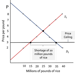
Price Controls:
Under a free market, theoretically, the consumer and producer surpluses are maximized. However, the government usually intervenes to regulate prices through price controls:
- Price Ceilings: are defined as the maximum price suppliers are allowed to charge for a good or service. A classic example of this is rent control.
- Price Floors: are defined as the minimum price consumers are required to pay for a good or service. A classic example of this is the minimum wage.

Imagine that the government decides to intervene in the market to protect consumers from price increases due to an enormous harvest failure in the rice fields. Thus, the government decrees a price ceiling so that the maximum price a producer can charge per pound of rice is $3 when the equilibrium price is $5. This will produce a rice shortage of 20 million pounds of rice. Figure 15 illustrates this scenario.
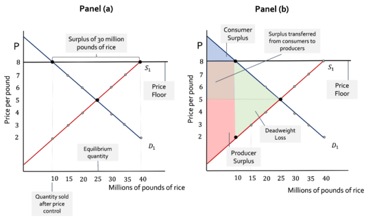
The shortage will create inefficiency in the market since the amount of rice transacted will be too low. Thus, there will be many consumers willing to buy rice who won’t’ be able to do it, and as a result, black markets are likely to appear. In this scenario, the total surplus will decrease, and the amount of the fall is called Deadweight Loss (DWL). Figure 16 illustrates it.
| Watch it |
|---|
Now, imagine an alternative scenario. The government would like to protect the producers from foreign cheaper rice. Thus, the government introduces a price floor so that the minimum price a pound of rice could be sold is $8 per pound. Similarly, this action will create inefficiencies in the market since it will create missing transactions among suppliers and lead to a surplus of 30 million pounds of rice in this market. Figure 17 illustrates this scenario.
Excise Taxes
Excise taxes are taxes on sales of goods and services used by the government to raise revenue. These taxes affect demand and supply because they increase the price consumers pay and reduce the price received by suppliers. Thus, we are usually interested in understanding who bears the tax burden or the tax incidence.
Tax on the Suppliers:
A tax on suppliers has the same effect as increasing the cost of production. Economists usually model this as if the supply curve shifted upwards by the amount of the tax.
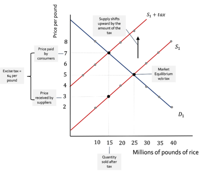
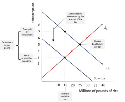
Figure 18 illustrates the effect of a tax on suppliers of $4 per pound of rice. The supply shifts down by $4, and the new equilibrium quantity is found where the demand and new supply meet.
Tax on the Consumers:
A tax on consumers has the same effect as decreasing their income. Economists usually model this as if the demand curve shifted downward by the amount of the tax.
Figure 19 illustrates the effect of a tax on consumers of $4 per pound of rice. The demand shifts down by $4; the new equilibrium quantity is found where the supply and new demand meet.
The anterior example illustrates that the tax incidence is the same regardless of whether the tax is on the sellers or the buyers. However, the tax division between consumers and suppliers will depend on the price elasticity of demand and supply. In the examples depicted in Figure 18 and Figure 19, consumers and suppliers paid the same amount in tax – i.e., $2, because the price elasticity of demand and supply is the same for both curves. However:
- When the elasticity of demand is higher than the elasticity of supply → the tax is paid mainly by the consumers.
- When the price elasticity of supply is higher than the price elasticity of demand → the tax is mainly paid by suppliers.
Efficiency

Imposing a tax usually creates inefficiency or DWL. Figure 20 illustrates the DWL, consumer surplus, producer surplus, and tax revenue when an excise tax is imposed on the supplier.
Marginal Benefit and Marginal Cost
The price found in free markets seems to coordinate individual actions in such a way that the outcome looks as if it were created by a benevolent invisible hand. However, even with a free market, the price sometimes isn’t right. To learn why the price isn’t always right, we must consider private and social costs and benefits.
| BENEFITS | COST | |
| PRIVATE | Received by the consumers or the producers in the rice market | Paid by the consumers or producers in the rice market |
| EXTERNAL | Received by people other than consumers and producers—those outside the rice market. | paid by people other than consumers and producers—those outside the rice market. |
| SOCIAL | Private + External | Private + External |
As a social planner, the government is interested in maximizing social surplus; thus, it needs to make sure it’s computing it correctly. To maximize social surplus, it needs to consider the private costs or benefits and the external ones. In particular, the government will pay close attention to Externalities.
An externality is a cost or benefit imposed onto a third party that isn’t directly related to the market where the externality is produced:
- External Cost: it’s a cost that an individual or a firm imposes on a third party and is not compensated. Externalities that impose external costs are called negative externalities; a classic example is air pollution.
- External Benefit: it’s a benefit that an individual or a firm grants to others without receiving any compensation. Externalities that confer an external benefit are called positive externalities, and vaccination is a classic example.
Externalities, then, produce social costs or benefits depending on whether they are negative or positive. So, the government will try to maximize:


To maximize social surplus, we must define:
- Marginal Private Cost (MPC): it’s defined as the additional private cost of producing one additional unit of a good or service as borne by the producer.
- Marginal External Cost (MEC): it’s defined as the additional cost of producing one additional unit of a good or service as borne by a third party unrelated to the producer.
- Marginal Social Cost (MSC): it’s defined as the additional cost imposed on society, including the one producing it and everyone else impacted, by producing one additional unit of a good or service. It’s equivalent to:
- Marginal Private Benefit (MPB): It’s defined as the additional benefit that a consumer of a good or service gets for consuming one additional unit of it.
- Marginal External Benefit (MEB): It’s defined as the additional gain that a third party gets from consuming one additional unit of a good or service.
- Marginal Social Benefit (MSB): It’s defined as the additional gain to society from consuming one additional unit of a good or service. It’s equivalent to:
