Documentation:CIS/iPeer/Coefficients

To setup iPeer coefficients, you can follow the guide below and refer to the video.

1. Download the iPeer data

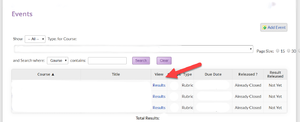
In iPeer, find the course and assignment you are calculating your coefficients for.

.....

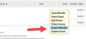
Right-click on the assignment and click "Export Results" .

.....

Give the CSV an appropriate name and download it.

Highlight the relevant data (Select cell A1 then use CTRL+SHIFT+DOWN ARROW).

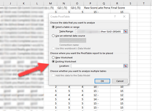
Select the "Insert" tab. Under the Pivot Chart dropdown arrow, select "Insert Pivot Chart and Pivot Table".

.....

We recommend placing the Pivot Table on the existing sheet.

.....

Delete the PivotChart by selecting it and pressing the delete key.

.....

Select "Group Name", "Evaluatee", "Evaluatee S#", and "Final Score" in the PivotTable fields.

.....

Move the Final Score field into the "Values" area.

.....

Select "Value Field Settings" on "Final Score".

.....

Choose "Average" under "Summarize value fields by".

.....

Switch to the "Show Values As" tab. Under "Show values as", scroll down and select "% of parent total".

.....

Select "Group Name" as the Base field.

.....

Your coefficients are now displayed in the "Average of Final Score" column in percentage form.

Go to the design tab while the PivotTable is selected.

.....

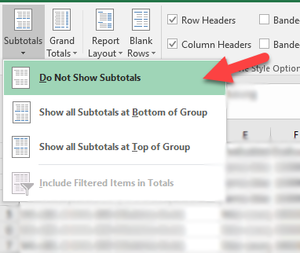
Under "Subtotals", select "Do Not Show Subtotals".

.....

Under "Grandtotals", select "Off for Rows and Columns".

.....

Under "Report Layout", select "Show in Tabular Form".

.....

Select the column containing coefficients and change the number formatting to "General".

.....

You can also select the data in the table and copy/paste it next to your existing data.