Course:MATH110/Archive/2010-2011/003/Teams/Zurich/Homework 11

To predict the cost of producing flags of our team’s Canton under the assumptions that the marginal cost is $7 per unit and that at the current production level of 20 items, the cost is $100, we wrote a linear model based on previous knowledge of revenue formulas:

$7 is the marginal cost, hence the slope = 7

The information above gives us the point (20,100)

• To find the linear equation, we substitute this point (20,100) into the equation y = 7x + b

100 = 7(20) + b

100 = 140 + b

b = 140 – 100 = 40

Therefore we get the equation:

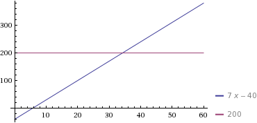
Y = 7x - 40, where x is number of units produced, and y is the cost

We can demonstrate this with the chart:

Based on this model, we can predict what it would cost for 150 items to be produced:

7(150) - 40 = 1010

• It would cost $1010 for the production of 150 items.

• Thus, according to this model, the average cost per item increases as production levels increase.

This is shown as 1010/150 = 6.73, whereas initially 100/20 = 5

Here are some other models related to this question:

The x-axis is Cost and the y-axis is the amount produced.

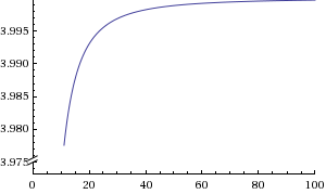
1) The average cost remains constant as production increases.

Y=((40x^4)+(4x^2))/((10x^4+8x^2))

when X goes to infinity, the graph would stay constant at y=4.

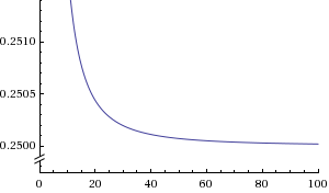
2) The average cost diminishes as production increases.

Y=((10x^4+8x^2))/ ((40x^4)+(4x^2))

when X goes to infinity, the graph would stay constant at y=1/4.

This could also interpreted as the fixed cost compound with variable cost where the graph can not go under the fixed cost.

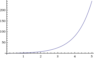
3) The average cost increases as production increases.

Y=3^(x)-1

As the production increase to a certain level, the marginal production will start to decrease and the marginal cost will start to increase. This is called law of diminishing return.

4)We obtain an economy of scale.

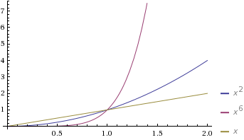
This means that starting at some specific production level, the marginal cost is always less than the average cost. This can be displayed in the following model:

As we can see in the model, y=x^2 represents the marginal cost, and y=x^6 represents the average cost. After production of 1, the marginal cost is always less than the average cost.

5)Interesting economic models.

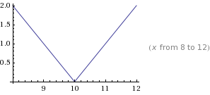
5a)V-shape recession

Y=|x-10|

In V-shape recession, an economy falls into a sharp recession but quickly recovers. A good example would be [recession of 1953] in United State.

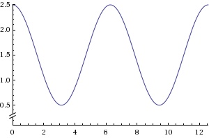
5b)W-shape recession

Y=Cos(x)+1.5

This is a well known "double-dipped" downturn.In a W-shaped recession, it would have a sharp downturn which is followed by small, temporary recovery.After the temporary "blip" in growth, the economy turns lower once again, before it eventually puts in a full recovery. A good example would be [Early 1980 recession] in United State.