Course:MATH110/Archive/2010-2011/003/Teams/Glarus/Homework 12

What we have to do:

modify the function so that we can use it to model a real-life problem. We want to be able to control the following things:

Change the height of the horizontal asymptote on the right, we'll denote it by K.

Change the y-intercept to any number between 0 and K

Change the slope of the curved part. Find a way so that the slope can go from very close to zero to almost vertical.

Information given:

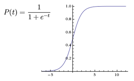
With the function P(t)= 1/1+e^-t we can modify it in a couple of ways. If we consider the function as P(t)= K/1+e^-t we can change the height of the horizontal asymptote on the right by setting K=whatever we want the horizontal asymptote on the right to be. The logic behind this involves considering the limit at +infinity. Horizontal asymptotes are limits at infinity. If we evaluate the limit at infinity for this function we find that it equals K.

Also, if we want to change the y intercept of the function then we can adjust A if we define the function as P(t)= 1/A+e^-t. At the y intercept t=0 so e^-t=1 so we get 1/A+1. This means we can adjust the y intercept to whatever we want because we just make A=whatever number we want minus 1.

We can now use this information to model something useful, like a population. We decided to model the population in Vancouver. For the sake of argument lets say that the carrying capacity of Vancouver is 1,000,000 people (a safe assumption since the biological definition of carrying capacity refers to the idea of the maximum population that an environment can support without habitat degradation and many people would argue that we're clearly already degrading the habitat and we're not yet at 1,000,000. If anything 1,000,000 would be well above carrying capacity but I digress...ANYWAY)

We want to find out in what year the population will reach 90% of its carrying capacity (in this case 900,000). According to trusty Wikipedia, the population of Vancouver was 578,041 people as of the 2006 census. Let's set that data point as our t=0. So our "Year 0" will be 2006 and so the y intercept will be 578,041 (the population at that time.)

P(t)= k/1+ae^(-rt)

k = Carrying capacity

a = Population at 0

r = Rate

t = x

We want to know when the population will reach 900,000 (90% of the carrying capacity). To determine this we can set P(t) as 900,000 and then evaluate for t.

To do this we need to figure out how much we need to shift our graph to the right so that the y intercept will be 578,041 and not halfway (500,000). To do this we have to find t when P(t)=578,041:

578,041= 10^6/1+e^-t

578,041 (1+e^-t)=10^6

1+e^-t = 10^6/578,041

e^-t=(10^6/578,041)-1

-t= ln [(10^6/578,041)-1]

-t=ln1.7-1

-t=0.7 -t=-0.3 t=0.3

So we need to shift our x coordinate 0.3 to the right for 578,041 to be our y intercept.

Now let's adjust the slope of the curved part by incorporating a specific rate of increase. According to worldometers.info the global population is increasing at a rate of 1.15%/year. Let's assume that since Vancouver is a smaller population to be drawing the percentage from that it is increasing slightly faster. Let's say that in 2006 the population was increasing at a rate of 2%/year. Since the population of Vancouver at that time was 578,041 the population would be increasing by 11,560.82 people that year (I know you can't have 0.82 of a person but let's just be accurate with our numbers and not round off at this point.) With our last variable r we have to determine what r is when the rate of change is 2%. To do this we have to a) find the derivative of the function so that we can model the rate of change b) set the derivative equal to 11,560.82 and solve for r (assuming t=0 because that's where P(t)=578,041)

P'(0)= [-(-re^(-rt+0.3)(10^6)]/(1+e^-rt+0.3)^2

11560=[-(-re^(-rt+0.3)(10^6)]/(1+e^-rt+0.3)^2

[(11560)(1+e^-rt+0.3)^2]/10^6= re^(-rt+0.3)

11560/10^6= (re^(-rt+0.3)/(1+e^-rt+0.3)^2

11560/10^6= [(r)(e^0.3)]/(1+e^0.3)^2

[(11560)(1+e^0.3)^2]/[(10^6)(e^0.3)]=r

0.047=r

So now our model is:

P(t)= 10^6/(1+e^(-0.047t+0.3))

We can determine when the population will reach 900,000 by evaluating P(900000) and solving for t.

900000=10^6/(1+e^(-0.047t+0.3))

We find that t=55.3 years Since our t=0 at 2006 we add 55+2006 to determine that the population of Vancouver will reach 90% of its carrying capacity during 2061.