^{Homework 11}

Model

At the current production level of 20 items the cost is 100 items and the marginal cost is $7 per unit.

When creating a graph of this model we can say that the x-axis refers to the number of items, and the y-axis refers to the cost of production. The marginal cost per each item is $7 so we can say that the slope at (20,100) is equal to 7.

We then can determine the equation of our model using slope-intercept form (y=mx+b).

In order to solve for "b" we substitute y and x for the values (20,100). For "m" we substitute in the slope which is 7.

We get:

       100= 7(20)+ b
       100= 140 + b
         b= -40

Since we know the value of "b" and "m" the equation of our model is: y= 7x-40 assuming y is greater than or equal to 20.

What does our model predict for a production of 150 items?

Since x= # of items produced, x=150. Therefore our model predicts:

y= 7(150)-40

y= 1050-40

y= 1010

Therefore our model predicts that for a production of 150 items, it costs $1010.

According to our model, what happens to the average cost per item as production levels increase?

Using our model we found that the average cost per item increases as production levels increase.

Since using the original values we were given (20,100), the average cost per item is $5.

Whereas the values we obtained for the production of 150 items (150,1010), the average cost per item is approx. $6.73

Examples of Other Models

1) Economies of Scale

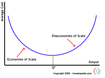
Economies of Scale mean the increase in efficiency of production as the number of goods being produced increases. Typically, a company that achieves economies of scale lowers the average cost per unit through increased production since fixed costs are shared over an increased number of goods.

"The more you buy, the more you save".

In this diagram, we see that as companies increase their production, this increase in production will lower the price and fixed cost which will in turn make more affordable products for consumers which will lead to higher market shares and revenue and more money to spend on production from the profits made and the cycle continues.

Larger companies and firms often are able to produce work more cost-efficiently than smaller ones. Economy of scale is when anything that you produce helps save costs if the scale of operation increases.

In this illustration you can see 'Output' on the x-axis and 'Average cost' on the y-axis. The long run average cost is depicted as the the rate of change as output increases and average cost is lowered. At Q outputs, your average cost is C, but when you increase your output to Q2, your average cost is C1 (economies of scale), therefore average cost continues to decrease as output increases to a certain point; approximately Q2, and then the more you make afterwards, will result in higher average cost (diseconomies of scale).

For example, larger companies have purchasing power to get better deals from supplies and lower cost of manufacturing because bigger factor have lower costs per unit produced. Larger companies also have better logistics leading to lower distribution cost.Economics of scale do not necessarily happen because a company is bigger. For example, you can combine two completely unrelated businesses together which is likely to lead to a higher costs by adding more management levels and worse management because you reduce focus on each business.

In retail stores, such as Superstore and Save-on-foods, the more orders of soft drinks the manufacturer receives, the more savings it makes, as it will in turn get cheaper prices for the materials it needs to produce its drinks (e.g. plastic, aluminium, sugar) as it will be buying them in larger quantities and receiving discounts, the manufacturing company in turn would give its customers cheaper prices for the more orders for drinks they make for this very reason, as they will gain the discounts, they can pass a saving onto their customers, making themselves stronger, a more respected company from its suppliers as it is buying in higher volumes and its turnover becomes higher. All these factors contribute to the benefits of economies of scale.

This is another illustration of the economies and diseconomies of scale. Economies of scale: when an increase in output leads to lower average cost (AC) and when to a certain point (Q* in this illustration), any further increase in output will lead to a higher AC.

2) Economic production quantity

Economic Production Quantity model (also known as the EPQ model) determines the quantity a company or retailer should order to minimize the total inventory costs by balancing the inventory holding cost and average fixed ordering cost. This method is an extension of the Economic Order Quantity model (also known as the EOQ model). The difference between these two methods is that the EPQ model assumes the company will produce its own quantity or the parts are going to be shipped to the company while they are being produced, therefore the orders are available or received in an incrementally manner while the products are being produced. While the EOQ model assumes the order quantity arrives complete and immediately after ordering, meaning that the parts are produced by another company and are ready to be shipped when the order is placed.

EPQ only applies where the demand for a product is constant over the year and that each new order is delivered/produced incrementally when the inventory reaches zero. There is a fixed cost charged for each order placed, regardless of the number of units ordered. There is also a holding or storage cost for each unit held in storage (sometimes expressed as a percentage of the purchase cost of the item).

We want to determine the optimal number of units of the product to order so that we minimize the total cost associated with the purchase, delivery and storage of the product

This is the Economic Production Quantity Model (EPQ model). This graph illustrates the total cost, the holding cost and the set up cost. On the x-axis, we have "Order quantity" and on the y-axis we have "Annual cost". This graph helps to determine the optimal number of units of the product to order so that we minimize the total cost associated with the purchase, delivery and storage of the product.