Course:CPSC522/Variable Elimination

Variable Elimination

Variable elimination(VE) is an algorithm to perform inference on Bayesian networks by manipulating conditional probabilities in the form of factors.

Principal Author: Ritika Jain

Collaborators: Tanuj Kr Aasawat, Prithu Banerjee

Abstract

The most common type of query we often need to find the probabilities for; is of the form P(Y|E=e) where Y is the set of variables that need to be queried and E is the set of observations we have made. This can be computed using any entry of the full joint probability distribution table, given the conditional probability tables in the network and then do inference by enumeration as shown below.

Given

a prior joint probability distribution(JPD) on a set of variables X.

specific values 'e' for the evidence variable E (subset of X).

We need to compute

posterior joint distribution of query variables Y (a subset of X) given evidence 'e'.

Method

Step 1: condition to get distribution P(X|e).

Step 2: marginalize to get distribution P(Y|e).

However, this method is extremely inefficient and does not scale well. We can perform better by taking advantage of variables independence. We can represent the joint probability distribution as a product of marginal distributions and simplify some terms when the variables involved are independent or conditionally independent.

Background knowledge

To understand variable elimination, we will first introduce the concept of factors and understand the operations that can be performed on them. This will be followed by the variable elimination algorithm, explained with an example.

Factors

A factor is a function from a tuple of random variables to the real numbers R We write a factor on variables X₁,… ,X_j as f(X₁,… ,X_j) A factor denotes one or more (possibly partial) distributions over the given tuple of variables, e.g., P(X1,X2) is a factor f(X1,X2). We shall look at three basic operations on factors: assigning a variable, summing out a variable and multiplying factors.

Assigning a variable

We can assign values to some or all variables of an existing factor to create a new factor.

The value of variables which are not satisfied are not considered in the new factor.

Summing out a variable

We can marginalize out (or sum out) a variable. Marginalizing out a variable X from a factor f(X₁,...,X_n) yields a new factor defined on {X₁,...,X_n} \ {X}

Multiplying factors

Two factors can be multiplied on the basis of a common variable to get a new factor. The product of factor f₁(A,B) and f₂(B,C) where B is the variable in common, is the factor (f₁ x f₂)(A,B,C) defined by: (f₁ x f₂)(A,B,C) = f₁ (A,B) f₂(B,C). The domain of f₁ x f₂ is AυBυC. This is shown in the figure below.

Introduction

We can express the joint probability as a factor of observed variables and other variables not involved in the query. f(Y, E₁,...,E_j, Z₁,...,Z_k). E's are the observed variables and Z's are the other variables not involved in the query. We can compute P(Y, E₁=e₁,....,E_j=e_j) by assigning E₁=e₁,....,E_j=e_j and marginalizing out variables Z₁,...,Z_k one at a time. This is represented as:

The order in which the marginalization of variables is done is called the elimination order. Finding the optimal elimination order is a NP complete problem.

We know the joint probability distribution of a Bayesian network as:

We can express the joint factor as a product of factors, one for each conditional probability.

Inference in Bayesian networks thus reduces to computing the above sum of products. This can be easily computed by

• partitioning factors into those that contain a particular 'Z_k' and that do not.
• summing out 'Zk' over all the factors that contain 'Z_k'. We explain this by the following example.

In the example above, we initially have four factors f1(C,D), f2(A,B,D), f3(E,A) and f4(D). We have one unobserved variable A that we need to sum over. We partition the factors into the sets that contain A: f2(A,B,D) and f3(E,A) and that do not contain a: f1(C,D) and f4(D). We sum over only the factors that contain A. From previous operation of multiplication of factors, we compute a new factor f5(A,B,D,E). Summing out the variable A, we get a new factor f6(B,D,E).

General case

Decomposition of sum of products can be seen as a general case as follows:

Algorithm

To compute the conditional probability P(Y=y_i | E=e), where E are the observed variables and Z are the variables not involved in the query, variable elimination algorithm[1] dictates as follows: 1. Construct a factor for each conditional probability. 2. For each factor, assign the observed variables E to their observed values

3. Given an elimination ordering, decompose sum of products.

4. Sum out all variables Z_i not involved in the query.

5.Multiply the remaining factors.

6. Normalize by dividing the resulting factor f(Y) by Σ_yf(Y) over all y.

Example

Consider the following Bayesian network and the query P(G | H=h₁). We consider a given elimination order A,C,E,I,B,D,F.

Essentially we need to compute Σ_{A,B,C,D,E,F,I}P(A,B,C,D,E,F,G,H,I). We sum over all the variables not involved in the query-A,B,C,D,E,F,I. Considering Bayesian independence, i.e., the current node depends only on its parent node, we can rewrite the above summation as:

$P(G,H)=\sum _{A,B,C,D,E,F,I}P(A)P(B|A)P(C)P(D|B,C)P(E|C)P(F|D)P(G|F,E)P(H|G)P(I|G).$

Step 1: Construct a factor for each conditional probability.

Writing the probabilities as factors we get,

$P(G,H)=\sum _{A,B,C,D,E,F,I}f_{0}(A)f_{1}(B|A)f_{2}(C)f_{3}(D,B,C)f_{4}(E,C)f_{5}(F,D)f_{6}(G,F,E)f_{7}(H,G)f_{8}(I,G).$

Step 2: Assign to observed variables their observed values.

We start by observing H=h₁ as given in the query which changes the factor f₇ to f₉. Therefore we get,

$P(G,H=h_{1})=\sum _{A,B,C,D,E,F,I}f_{0}(A)f_{1}(B|A)f_{2}(C)f_{3}(D,B,C)f_{4}(E,C)f_{5}(F,D)f_{6}(G,F,E)\color {red}{f_{9}(G)}\color {black}{f_{8}(I,G).}$

Step 3: Decompose sum of products.

According to the elimination order provided to us, we need to perform product and sum out A first, then C, then E and so on. All factors involving A will be considered in the summation of A as shown below:

$P(G,H=h_{1})=f_{9}(G)\sum _{F}\sum _{D}f_{5}(F,D)\sum _{B}\sum _{I}f_{8}(I,G)\sum _{E}f_{6}(G,F,E)\sum _{C}f_{2}(C)f_{3}(D,B,C)f_{4}(E,C)\color {blue}{\sum _{A}f_{0}(A)f_{1}(B|A)}.$

Step 4: Sum out non query variables (one at a time).

Performing product of f₀(A) and f₁(B,A) we get, f₁₀(B,A). Summing out A, we get f₁₁(B). This factor will be considered under the summing variable B as it does not depend on C,E,I (according to the elimination order) and therefore will be pushed outside of these sums.

$P(G,H=h_{1})=f_{9}(G)\sum _{F}\sum _{D}f_{5}(F,D)\sum _{B}\color {red}{f_{11}(B)}\color {black}{\sum _{I}f_{8}(I,G)\sum _{E}f_{6}(G,F,E)\sum _{C}f_{2}(C)f_{3}(D,B,C)f_{4}(E,C).}$

Performing the product and summing out C, we get the factor f₁₂(D,B,E). This factor will be pushed under the summation of E as E comes before B and D in the elimination order.

$P(G,H=h_{1})=f_{9}(G)\sum _{F}\sum _{D}f_{5}(F,D)\sum _{B}f_{11}(B)\sum _{I}f_{8}(I,G)\sum _{E}\color {blue}{f_{12}(D,B,E)}\color {black}{f_{6}(G,F,E).}$

Similarly multiplying f₁₂(D,B,E)f₆(G,F,E) and summing out E, we get the factor f₁₃(B,D,F,G),

$P(G,H=h_{1})=f_{9}(G)\sum _{F}\sum _{D}f_{5}(F,D)\sum _{B}f_{11}(B)\color {red}{f_{13}(B,D,F,G)}\color {black}{\sum _{I}f_{8}(I,G).}$

Continuing on these lines, we finally end up with; $P(G,H=h_{1})=f_{9}(G)f_{14}(G)f_{17}(G).$

Step5: Multiply remaining factors.

Multiplying all the remaining factors in G, we get,

$P(G,H=h_{1})=f_{18}(G)$

Step 6: Normalize

$P(G=g|H=h_{1})={\frac {P(G=g,H=h_{1})}{\sum _{g'\in dom(G)}P(G=g',H=h_{1})}}={\frac {f_{17}(g)}{\sum _{g'\in dom(G)}f_{17}(g')}}$

Further optimizations

In the previous example we did not take advantage of the conditional independence in the Bayesian network.

1. Conditional Independence:
   Before we run variable elimination, we can reduce the nodes we need to consider by pruning all variables Z that are conditionally independent of the query Y given evidence E: Z $\perp \!\!\!\perp$ Y | E.
   Example: Considering the same Bayesian network, for the query P(G=g | C=c₁, F=f₁, H=h₁); we can prune elements A,B and D because both paths from these nodes to G are blocked.
   
   • F is observed node.
   • C is an observed common parent.
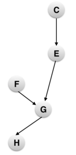
2. Unobserved Leaf Nodes:
   We can also prune the unobserved leaf nodes since they are unobserved and also not the predecessors of the query nodes, they will not have any effect on the posterior probability of the query nodes.Therefore in the above example, we can prune variable I. We only need to run Variable Elimination on this reduced subnetwork as shown below.
   
   This makes the entire process more efficient and reduces the runtime complexity.

Complexity

A factor over n binary variables needs to store 2ⁿ numbers. The initial factors are usually small because variables have only a few parents in the Bayesian network, but after product, the factors tend to get large. The complexity of Variable Elimination is exponential in the maximum number of variables in any factor during its execution. This is also called the treewidth of a graph (along a particular variable elimination order). Finding the most optimal variable elimination order (i.e the one which gives the minimum treewidth) is NP complete. However, heuristics such as ordering the least connected variables first work well in practice.

AISpace Demo

End of civilization? or Not?

We look at a demo example from AISpace[2] which uses variable elimination to answer some interesting questions- Is it the end of civilization?

The scenario is: Bill has noticed that his morning newspaper delivery has been sporadic. There are several relevant variables relating to whether or not the paper is delivered. Delivery is dependent on the paper having been successfully printed the previous night. Possible explanations for a paper not having been printed are a malfunction at the printing press, or the end of civilization as we know it.

The probabilities assigned are: The prior probability of a printer malfunction is 0.05. Bill has been noticing some ominous signs of the apocalypse and so expects the end of civilization with a relatively high probability of 0.001. If the end of civilization is here, then the paper not be printed for sure. If there is a printing malfunction and no end of civilization, there is a probability of 0.05 that the paper will be printed (this is non-zero because the malfunction might be fixed in time). If there is no malfunction and no end of civilization, there is a probability of 0.99 that the paper will be printed. If the paper is not printed it will not be delivered. If it is printed, there is a probability of 0.9 that it will be delivered. The fact that this probability is not 1 suggests that there are other possible causes for the paper not being delivered that we should eventually add to our belief network (e.g. the paperboy being sick). A short demo[3] that I have created can be viewed here:

Applications

Variable elimination[4] is a general technique for constraint processing. When combined with other techniques, it can be extremely useful for solving many problems arising in domains such as resource allocation, combinatorial auctions, bioinformatics and probabilistic reasoning that can be naturally modelled as constraint satisfaction and optimization problems. Finding the posteriori belief has multiple applications in statistical analysis and learning. Given a causal trail, calculating the conditional probability of effects given causes is called prediction. In this case, the query node is a descendant of the evidence. Diagnosis is calculating the conditional probability of causes given effects, and this is useful in finding the probability of a disease given the symptoms. In this case, the query node is an ancestor of the evidence node in the trail. While learning under partial observation, posteriori belief of the unobserved variables given the observed ones is calculated. Variable elimination works equally well for both Bayesian networks and Markovian networks.

Annotated Bibliography

1. David Poole & Alan Mackworth, "Artificial Intelligence: Foundations of Computational Agents",
2. AISpace
3. Youtube demo
4. CMU lecture notes

To add

-Link to Bayesian network -