Course:CPSC522/The Automation of Disease Diagnosis

Title

This page presents the application of L1 regularzied SVM in feature selection of some disease data sets.

Principal Author: Ke Dai

Abstract

Figure 1 Machine learning in disease diagnosis

Machine learning has been widely used for intelligent data analysis in the domain of medical and health service. A tremendous amount of patient information including medical images, various physiological indexes, coupled with other details like age, height, weight, and medical history provides abundant data resources to analyze, screen and mine data and thus to extract valuable information from these data. Medical and health organizations can make use of data mining techniques to analyze the root or law of diseases, thus discovering better treatment and improving effectiveness of curing. In the process of medical diagnosis, the application of data mining techniques render it possible to effectively process massive historic data in the database of patient information and to explore worthy law of medical diagnoses, which enables doctors to make reliable diagnoses more confidently based on the results of physical examination and the variation of physiological indexes. This increases the efficiency and quality of diagnoses significantly, makes diagnoses more objective and convincing. However, many disease data sets include too many features, some of which may be redundant or irrelevant. Using these data sets to train a learning model significantly deteriorate the generality, performance and explainability of the model. As a result, it is absolutely essential to conduct feature selection before data mining. This page presents the performance of L1 regularization in feature selection when applied in some disease data sets.

Builds on

This page builds on Feature Selection, Regularization, SVM, L1-norm SVM.

Content

Introduction

In medical diagnosis, applying data mining techniques to explore valuable law of diagnosis from massive historic data of patient information makes possible the automation of medical diagnosis based on the age, gender, the results of physical examination and physiological indexes of a patient, thus preventing the interference of subjective factors and making the diagnosis more objective and convincing. Since the law of diagnosis is derived from a large amount of data, the rules of diagnosis have great generality. For example, Georgia Tourassi, a data scientist at the Oak Ridge National Lab, used 1064 patient cases (383 with pulmonary embolism, 681 without pulmonary embolism) to train and test an ANN (artificial neural network), and compared the diagnoses of ANN with the diagnoses of an physician. The result proved that ANN has higher accuracy.

However, the application of machine learning in medical data mining is also faced with some challenges. One of them is that medical databases contains a great amount of original data with different sources, many of which are ambiguous, incomplete, noisy or redundant. Before conducting data mining, it is essential to perform data cleaning and screening to ensure the consistency and correctness and then to transform the original data to standard format applicable to mining. Meanwhile, the data may include too many features. Some of these features are redundant or irrelevant to the learning objective. The existence of these redundant features not only degenerate the generality and performance of program, but also weakens the explainablity and understandability of the model.

Hypothesis

I want to conduct feature selection in some disease data sets collected from the internet using L1 regularization, a well-known method of feature selection. Does it really work on these disease data sets? Does it keep, increase or decrease predictive accuracy using new data sets to train the learning model after feature selection? To answer these questions, I will train the learning model on original data sets and new data sets after feature selection using the same machine learning algorithm, and compare predictive accuracy of the learning model.

Background Knowlege

Feature Selection

Why do we need feature selection?

Feature selection is a very practical technique whose objective is to eliminate the noise in the data before data mining. As human beings, when we discern the class of an object, we always make a judgement based on our experience or some information of the object. For example, to judge the brand of a car, we prefer to draw the conclusion according to the logo because this is the most straightforward and persuasive information of a car to judge its brand. But if we make a judgement based on the appearance of the car, we may take a Benz as an Audi wrongly. That is to say, we human beings always select the most valuable information to make our judgement.

However, computers cannot select the most effective information according to experience like human beings when being faced with similar problems. As a result, a large amount of redundant or irrelevant information is noise for computers and will exert a negative effect on the judgement of computers. Feature selection aims to select the most relevant features with the learning objective and thus to improve predictive accuracy. Meanwhile, feature selection also enhance the performance and explainability of the learning model.

What is feature selection?

• General Definition

Feature selection, also known as variable selection, attribute selection or variable subset selection, is the process of selecting a subset of relevant features (variable, predicators) for use in model construction.

• Formal Definition

Figure 2 The process of feature selection

Feature selection is to find a subset consisting of M features selected from the originally given N features such that this subset is the optimal subset among all the subsets consisting of M features in terms of a certain evaluation criterion.

• Definition from the perspective of predictive accuracy

Feature selection is to find a subset of features to improve predictive accuracy or reduce the dimensionality of the set of features without weakening predictive accuracy.

Feature selection is essentially a combinatorial optimization problem. To solve the combinatorial optimization problem, the most straightforward method is searching. In principle we can traverse all possible combinations by exhaustive search to find the optimal combination of features as the output in terms of a given evaluation criterion; however, computation cost increases exponentially with the dimensionality of features as the search space for n features is $2^{n}$. A large amount of data contain hundreds and even thousands of features in reality, so exhaustive search is impractical though simple. Two other alternative methods are heuristic search and random search, both of which aim to trade off the quality of the subsets and computation complexity.

How can we perform feature selection?

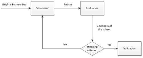
The general process of feature selection is comprised of 4 basic steps including generation procedure, evaluation function, stopping criterion, and validation procedure shown in Figure 2. First, a candidate subset of features is generated from the whole set in generation procedure, and then evaluated with evaluation function. The evaluation result is compared with the stopping criterion to decide whether to stop the process of feature selection or not. If the evaluation result meets the stopping criterion, the process of feature selection stops, else the process is repeated until a subset of features meeting the stopping criterion is found.

Regularization

Figure 3 Ground Truth Fit Model

Figure 4 Overfitted model

Motivation

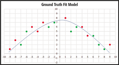
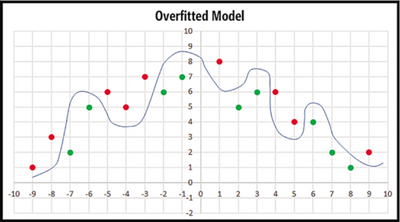
Regularization, in mathematics and statistics and particularly in the fields of machine learning and inverse problems, refers to a process of introducing additional information in order to solve an ill-posed problem or to prevent overfitting. Before we get into regularization, let's first have a look at what is overfitting by Figure 4 and Figure 5. We can see that the curve separates most of red and green points in Figure 4 but there are still two red points and two green points separated on the wrong side while the curve separates all the points in Figure 5. Which one is better? The answer is the curve in Figure 4. Although the curve in Figure 5 has better predictive accuracy on training Data, predictive accuracy may be bad when we apply it in new data as it is irregular. This is called overfitting. Overfitting occurs where the magnitude of weights are very large. Therefore, one way to reduce overfitting is to prevent model weights from becoming very large. This is the motivation for regularization.

L1 and L2 Regularization

When a machine learning model is trained, we always use some error function to evaluate the performance of the model. One frequently used error function is the mean squared error. Take logistic regression for example. Suppose we have n samples in a dataset and every sample has an expected output and an actual output value by our model, the mean squared error can be expressed as:

${\frac {\sum _{k=1}^{n}(t-o)^{2}}{n}}$

where t represents the desired output value of every sample, t is the actually computed output value of every sample. So the learning objective of our model is to find a set of weight values which minimize the value of the error functions. As mentioned above, Large magnitude of weights may lead to overfitting. An ingenious method to prevent weights from becoming very large is including the values of weights in the error function so that large weight values generate large error values.

There are two kinds of regularization based on the form of included weight values. One is called L1 regularization which includes the sum of absolute values of weights in the error function. It can be expressed as:

${\frac {\sum _{k=1}^{n}(t-o)^{2}}{n}}+\sum |w_{i}|$

The other is called L2 regularization which includes the sum of squared values of weights in the error function. It can be expressed as:

${\frac {\sum _{k=1}^{n}(t-o)^{2}}{n}}+{\frac {1}{2}}\sum w_{i}^{2}$

Both L1 and L2 regularization can prevent the overfitting of a learning model efficiently. However L1 regularization has a beneficial side effect of generating a sparse matrix of weights which is characterized by many weights with zero value. This is great because it means the corresponding features do not contribute to the output. Consequently, L1 regularization can also be used for feature selection.

Support Vector Machine

Figure 3 Support Vector Machine

Principle

SVM (Support vector machine) is a supervised model in machine learning. It can generally be used in pattern recognition, classification, and regression, and is considered as the best stock classifier by some people as even the basic form of SVM can achieve the low error rate.

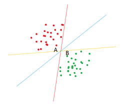
Before getting into SVM, let's first have a look at the linear classifier. Given a set of data points which belong to two classes, we want to find a linear classifier to seperate these data. If the data points are denoted by x and the classes (1, -1) are denoted by y, the learning objective of a linear classifier is to find a optimal hyper plane in the n-dimension space. This hyper plane can be denoted by the equation $w^{T}x+b$. In fact, there may be an infinite number of hyper planes which can divide these data into two classes, but which one is the best? SVM tries to find the hyper plane which has the farthest distance from the nearest points. These points are called support vectors. To be more intuitive, let's look at Figure 3. You can see that all three lines can seperate red points and green points, but which one is better? From SVM's perspective, the blue one is better thant the other two as it has the farthest distance from the nearest points A and B. To get the optimal hyper plane, we must calculate the distance between support vectors and the hyper plane, which can be denoted by $|w^{T}A+b|/||w||$.

Apply sign function as the activation function of $w^{T}x+b$, so we can get a class label +1 when $w^{T}x+b>0$, and -1 otherwise. Here we use -1 and 1 as class labels because this way makes it convenient to calculate the distance between points and the hyper plane. Considering the equation $label\cdot (w^{T}x+b)$ we use to calculate the distance, it always evaluates to a positive number whether the label of the data is 1 or -1. So we can use one uniform equation to calculate the distance for data of both labels.

Now the goal is to find the values of w and b. First, we must find the points with the smallest distance, and then we need to maximize the distance. It can be summarized by an equation like this:

$argmax_{w,b}{\bigg \{}min_{n}(label\cdot (w^{T}x+b))\cdot {\frac {1}{||w||}}{\bigg \}}$

To solve this problem directly is very difficult, so we transform it to another form which can be solved more easily. As optimizing the multiplication is very hard, we assume the values of $label\cdot (w^{T}x+b)$ for all support vectors are 1 and thus we can solve this problem by searching the maximum $||w||^{-1}$. So now this problem is an optimization problem given the constraint that $label\cdot (w^{T}x+b)\geq 1$. For this kind of constraint optimization problem, a well-known method is using Lagrange multipliers. By Lagrange multipliers, we can decribe this problem based on the constraint. As a result, the optimization function can be written as:

$max_{\alpha }{\bigg [}\sum _{i=1}^{m}\alpha -{\frac {1}{2}}\sum _{i,j=1}^{m}label^{(i)}\cdot label^{(i)}\cdot a_{i}\cdot a_{j}\left\langle x^{(i)},x^{(j)}\right\rangle {\bigg ]}$

The constraint is

$\alpha \geq 0$, and$\sum _{i=1}^{m}\alpha _{i}\cdot label^{(i)}=0$

This optimization function is built on the assumption that all data are linearly separable; however, in reality this assumption is too ideal. So we introduce a slack variable to allow some data to be on the wrong side of the hyper plane such that we still have the same optimization function but the constraint is changed to:

$C\geq \alpha \geq 0$, and$\sum _{i=1}^{m}\alpha _{i}\cdot label^{(i)}=0$

Here the constant C is used to control the maximum distance and to ensure most of the points have a distance of greater than 1 from the hyper plane. When implementing this optimization algorithm, we can tune the value of C to get different results. Once all alphas are got, the hyper plane can be expressed in terms of alphas. This conclusion is very straightforward, so all we need to do is to find all alphas.This is just the fundamental principle of SVM and actually the implementations of SVM have some improvements based on this idea.

Dataset Preparation

I got three datasets from KEEL dataset website. They are heart, thyroid and hepatitis respectively. Every dataset is divided into to two parts. One is used as the training dataset (80%) and the other is used as the test dataset (20%).

• Heart

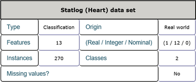
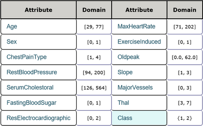
This is a heart disease data set including 13 features and 1 class label. The features consist of age, sex and other physiological indexes among which one feature is real numbers and the others are integer numbers. There are 270 instances in total and there are no missing values in this data set. Every sample belongs to one of two classes which represent the absence and presence of heart disease in the patient respectively. Detailed inforamtion is shown in Table 1 and Table 2. The task is to detect the presence of heart disease in the patient according to every patient's physiological indexes.

General information

Table 1 General information for heart dataset

Attribute description

Table 2 Attribute description for heart dataset

• Thyroid

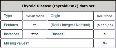
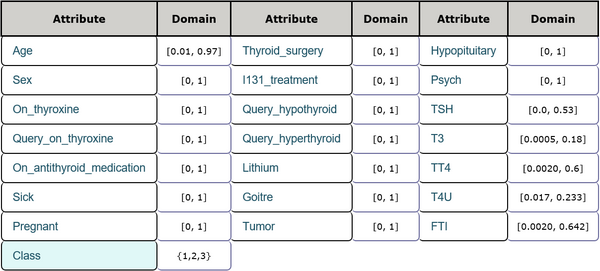
This is a thyroid disease data set including 21 features and 1 class label. The features consist of age, sex and other physiological indexes among which 6 features are real numbers and the others are integer numbers. There are 7200 instances in total and there are no missing values in this data set. Every sample belongs to one of three classes which represent that a given patient is normal, suffers from hyperthyroidism, or hypothyroidism. Detailed inforamtion is shown in Table 3 and Table 4. The task is to detect the presence of thyroid disease in the patient according to every patient's physiological indexes.

General information

Table 3 General information for thyroid dataset

Attribute description

Table 4 Attribute description for thyroid dataset

• Dermatology

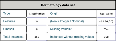
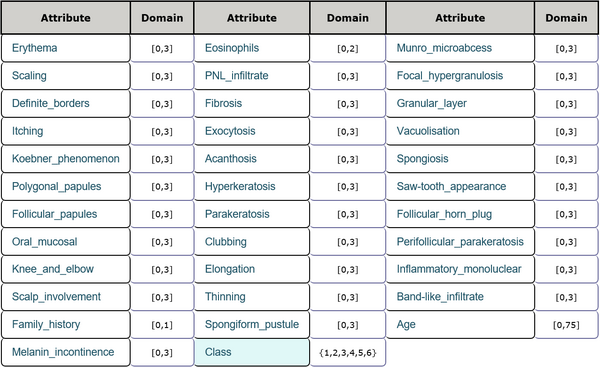
This is a dermatology data set including 34 features and 1 class label. The features consist of age, family history and other physiological indexes all of which are integer numbers. There are 366 instances in total and 358 of them are without missing values. Every sample belongs to one of the six classes. Detailed inforamtion is shown in Table 5 and Table 6.

General information

Table 5 General information for dermatology dataset

Attribute description

Table 6 Attribute description for dermatology dataset

Test Results

I used Python to implement the L1 regularized SVM model and train the model on all these datasets and new datasets after feature selection.

• Heart

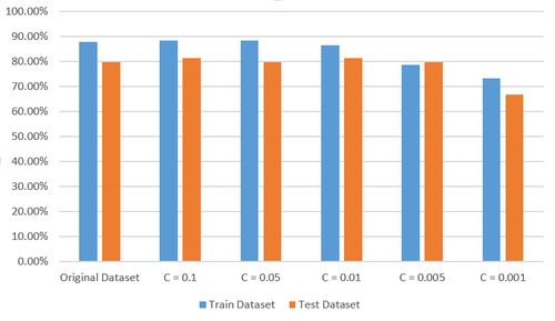
When I trained the model with the original heart data set, predictive accuracy of the model on training data set attains 87.96% while preditive accuracy on testing data set is 79.63%. Then I tuned the value of parameter C in the optimization function of L1 regularized SVM to 0.1, 0.05, 0.01, 0.005, 0.001 to conduct feature selection on the original data set respectively. Here I want to explain the parameter C briefly. C is the penalty coefficient of error which represents to what extent you are tolerant to the error. The bigger the value of C is, the less tolerant you are to the error. That is to say, a too big value of C gurantees better predictive accuracy but may lead to overfitting while a too small value of C leads to bad predictive accuracy. So you have to find an approriate value of C by trial in practice.

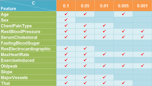
When C is set to 0.1, only FastingBloodSugar and Slope features were removed and the model achieved predictive accuracy of 88.43% and 81.48% on the new training data set and testing data set respectively. When C is set to 0.05, one more feature Sex was removed and the model achieved predictive accuracy of 88.43% and 79.63% on the new training data set and testing data set respectively. When C is set to 0.01, three more features Age, ResElectrocardiographic and ExerciseInduced were removed and the model achieved predictive accuracy of 86.57% and 81.48% on the new training data set and testing data set respectively. When C is set to 0.005, two more features ChestPainType and MajorVessel were removed but Age is retrieved and the model achieved predictive accuracy of 78.70% and 79.63% on the new training data set and testing data set repectively. When C is set to 0.001, only four features RestBloodPressure, SerumCholestoral, MaxHeartRate, Oldpeak were selected while there is a significant decrease in predictive accuracy which is 73.15% and 66.67% on the new training data set and testing data set repectively. So 0.005 is a safe value of C to get the sufficient and necesssary subset of features and all these features are very important for the learning objective.

Figure 6 Comparison of predictive accuracy for heart dataset

Figure 7 Selected features with different values of C for heart dataset

• Thyroid

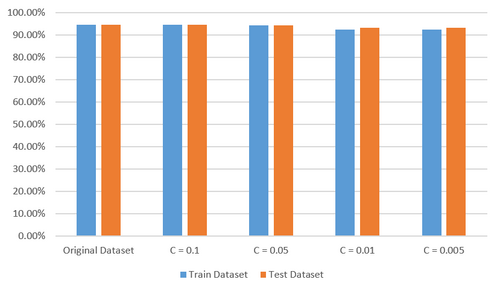
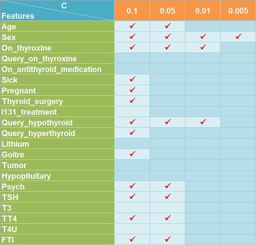
For thyroid data set, I conducted similar procedures to that of heart data set. From Figure 9, we can see that predictive accuracy of the learning model on all the data sets attained more than 90 percent. However, the result is not optimistic but anomalous considering only the feature Sex is selected when C is set to 0.05 shown in Figure 8 as you must think it is ridiculous if someone tells you whether a patient suffers from thyroid disease can be predicted only according to his or her sex. So I tried to find the cause of this problem. It seems explainable when I found that most of the samples in the original data set belong to class 3 which represents a patient suffers form hypothyroidism. That is to say, even if the model wrongly take samples of class 1 and class 2 as class 3, it will not have a significant effect on predictive accuracy of the model.

Figure 8 Comparison of predictive accuracy for thyroid dataset

Figure 9 Selected features with different values of C for thyroid dataset

• Dermatology

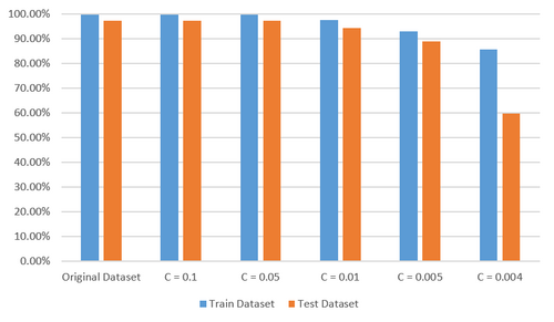
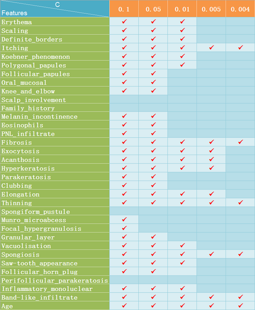
For dematology data set, I just repeated the previous process of experiment. From Figure 10 and Figure 11, we can see that 6 features are selected when C is set to 0.004 and there is a distinct decrease in predictive accuracy of the model trained with this new data set with only 6 features while it is relatively safe to set the value of C to 0.005 with which 10 features are selected without significant loss of predcitive accuracy. Considering there are 34 features in the original data set, it is not a bad result.

Figure 10 Comparison of predictive accuracy for dermatology dataset

Figure 11 Selected features with different values of C for dermatology dataset

Conclusion and Future Work

From the experiment results, we can find when tuning C to an appropriate value, we can always get a sufficient and neccessary subset of features with which the learning model can be trained to attain equivalent preditive accuracy to that of the learning model trained with the original data set. L1 regularized SVM performs well on all the three data sets; however, the result for thyroid data set is not resonable as most samples in the data set belong to one class. Meanwhile, it also demonstrates that the distribution of samples of different classes in a data set is very important. The imbalanced distribution of samples will misdirect feature selection and even make the learning model meaningless. On the other hand, I only conducted feature seletion on three disease data sets due to time constraint. As a result, in the future I will collect more data sets with good distribution to conduct feature selection and I believe more problems will be found with more data sets. Meanwhile, I will also explore other possible methods of feature selection and compare the performance of different methods.

To Add

Put links and content here to be added. This does not need to be organized, and will not be graded as part of the page. If you find something that might be useful for a page, feel free to put it here.