Course:CPSC522/Recursive Error Division Validation

Recursive Error Division Validation

Author: Celeste/Clair

Original code available here

Hypothesis

Since gender is often assumed to be a binary in many datasets it disrupts the validity of the claims and analysis of the data. It would be helpful to understand the impact of a feature of a dataset that is considered a socially constructed idea and how to better translate that into a countable and measurable domain.

I believe that if sub-datasets are constructed from the data that doesn't fit a given prediction threshold, and that the domain of the predicted value is treated like new unique values expanding the old domain, and that is this is iterated on, then either the predictions from the model should become more accurate or the feature should be considered less relevant with its original domain.

Background

Iterable Predictor

I will start with a dataset $S$ that has a gender feature with a domain with 2 values, $F$ and $M$. I then consider that, for some threshold $\gamma$, $0.5<\gamma <1$, if the probability of being either $F$ or $M$ is less than $\gamma$ then we add this item to a new set, which is a subset of $S$.

I will then iterate on this idea, letting $S_{i}$ be the set at the $i$-th iteration. The original $S$ is then $S_{0}$ and $S_{i+1}\subseteq S_{i}$.

In the set $S_{i}$, I then replace the values $F$ and $M$ with the new labels $g_{2i}$ and $g_{2i+1}$. The original values in $S_{0}$ are then $g_{0}$ and $g_{1}$. I then consider, for set $S_{i}$, a new domain of gender with all the gender values up to that iteration, $G_{i}=\{g_{0},...,g_{2i+1}\}$.

I allow that each iteration may use a consistent threshold $\gamma$ or varying thresholds $\gamma _{i}$ for finding the next subset $S_{i+1}$. If the next iteration's set is unchanged, that is $S_{i}\equiv S_{i+1}$, then all items passed the given threshold. If this occurs then I either need to end the iterations or increase the threshold $\gamma$.

For each iteration $i$, I consider a modified version of the original dataset $S$, where the gender value is replaced with it's value from $G_{i}$ which I call ${\hat {S}}_{i}$. I then use this dataset to predict the ratings of movies by users and compare those prediction accuracies.

Matrix Multiplication Predictor

The matrix multiplication predictor is written in the source as:

Matrix factorization techniques have proved effective especially in recommendation systems [Koren et al., 2009]. The idea is to factorize a relation matrix over two types of objects (e.g., users and movies) into latent features for each type of objects such that the relation matrix can be approximated using the latent features. Koren et al. [2009] use matrix factorization for movie recommendation and factorize the rating matrix as follows:

${\hat {R}}_{ui}=\mu +b_{u}+b_{i}+\sum _{f}P_{uf}\ast Q_{fi}$

where ${\hat {R}}_{ui}$ is the predicted rating of user $u$ for movie $i$, $\mu$ is a bias, $b_{u}$ and $b_{i}$ are user and movie biases, and $P_{uf}$ and $Q_{fi}$ are the $f$-th latent property of the user $u$ and movie $i$ respectively.

When the ratings are in binary (e.g., greater than equal to 4 or less than 4), the model can be trained to predict:

$P({\hat {D}}_{ui})=sigmoid\left(\mu +b_{u}+b_{i}+\sum _{f}P_{uf}\ast Q_{fi}\right)$

where $D_{iu}$ is true when the rating for user $u$ on item $i$ is 4 or greater and is false when it is less than 4. The same training algorithm as Koren et al. [2009] can also be used here to minimize log loss.

While matrix factorization method might not be new, it has not be used explicitly for aggregation.

One way to use matrix factorization for aggregation is to factorize the relation matrix into latent features, then use the latent features of the desired objects as features and build a model over these features to make predictions about them. For our running example, we train a logistic regression on $b_{u}$ and $P_{uf}$ for each $f$ to predict the gender of the users, which takes the following form:

$P(female(u)|b_{u},P_{u})=sigmoid\left(w+w'\ast b_{u}+\sum _{f}w_{f}\ast P_{uf}\right)$

where $P_{uf}$ is, as previously mentioned, the $f$-th latent property of the user u</math>. This was the method reported as “matrix factorization” in the results.

"Movie-as-a-dataset" Predictor

From the source paper for the predictors using each movie as it's own dataset to predict the probability of the binary gender. The equation is

$P_{1}(female(u)|E)={\frac {c+\sum _{\{i:rated(u,i)\}}\#u':rated(u',i)\wedge female(u')}{2c+\sum _{\{i:rated(u,i)\}}\#u':rated(u',i)}}(1)$

Here, $c$ is a parameter set by validation and is thought of as a pseudo-count. The sum is the count of users who rated the movie who both do and don't meet the condition (in this case, if the binary gender is "F"), and the sum is only taken over movies that have been rated by the predicted user $u$.

The paper specifically says:

A movie with $n$ ratings can be seen as $n$ data points about the users who rated this movie. The idea behind this approach is similar to rule combining of Natarajan et al. [2008], where each parent independently predicts the target and then these independent predictions are combined. However, we do not tie the parameters for parents, and we do not consider intermediate hidden variables for each parent’s prediction that should be learned using EM. One way this can be used is to use all of the people who rated the movies that $u$ rated:

(1) from above.

Where the denominator only includes ratings by users whose gender is known, and $c$ is a pseudo-count (beta/Dirichlet prior), which is set in our experiments by 5-fold cross validation (and was often quite large). Counting only the users that rated the same as $u$ worked slightly worse (presumably because there were fewer datapoints for each user). Using more informed prior counts (which predict the training average for users that rated no movies) also worked worse. We will not consider these variants here.

Methods

While I wanted to implement all the predictors in the provided paper[cite], I was only able to add one additional: Movies as a dataset (Eq (6)).

With this additional predictor I had the following:

• Matrix Multiplication Predictor
• 0.5 Predictor
• Average Predictor
• "Movies-as-a-dataset" predictor

I then implemented the iterative predictor generator described above to create ${\hat {S}}_{i}$. Due to time constraints I was unable to put together the finished product that would take the modified set of users with the new gender set and predict movie ratings.

Instead, I plotted the probabilities of the training data with each predictor and then sorted the values for readability. Then, using this chart, I selected reasonable $\sigma$ tolerances and, for both matrix multiplication and "movies-as-a-dataset" predictors, I compared the iterations against each other.

Finally, I returned to the probability distribution of each predictor, but this time, comparing each iteration against each other.

Results

Prediction spread

I plotted the probability predictions using four predictors:

• Matrix Multiplication Predictor
• 0.5 Predictor
• Average Predictor
• "Movies-as-a-dataset" predictor

Prediction spread of four predictors: Matrix multiplication predictor, 0.5 predictor, average predictor, and "movies-as-a-dataset" predictor.

The matrix multiplication predictor

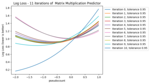
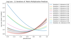
The matrix multiplication predictor had the most "sigmoid-like" distribution, so I began by choosing a few different tolerances. I used 2 consistant tolerances $\sigma =0.95$ and $\sigma =0.99$;

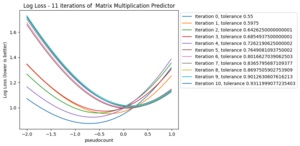
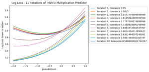
Then I used an ascending and descending tolerances $\sigma _{i}=0.95^{i+1}$ and $\sigma _{i}=1.5-0.95^{i+1}$ respectively for $i=\{0,...,10\}$.

Log loss on 10 iterations of the matrix multiplication predictor with tolerance $\sigma =0.95$

Log loss on 10 iterations of the matrix multiplication predictor with tolerance $\sigma =0.99$

Log loss on 10 iterations of the matrix multiplication predictor and an ascending tolerance $\sigma _{i}=0.95^{i+1}$

Log loss on 10 iterations of the matrix multiplication predictor and a descending tolerance $\sigma _{i}=1.5-0.95^{i+1}$

Table 1: Minimum Log Loss along iterations of Matrix Multiplication Predictor with different tolerances

Tolerance model	Iteration 0	Iteration 1	Iteration 2	Iteration 3	Iteration 4	Iteration 5	Iteration 6	Iteration 7	Iteration 8	Iteration 9	Iteration 10
$\sigma =0.95$	0.87443	0.89299	0.94289	0.91167	0.84172	0.78529	0.75468	0.46494	0.63983	0.79911	0.90502
$\sigma =0.99$	0.87443	0.91411	0.95918	0.95350	0.97569	0.96704	0.98397	0.95252	0.98378
$\sigma _{i}=0.95^{i+1}$	0.87443	0.80259	0.81235	0.96598	0.91578	1.01152	1.01276	1.01148	1.01523	1.02503	1.02025
$\sigma _{i}=1.5-0.95^{i+1}$	0.87443	0.87671	0.91126	0.92439	0.78847	0.79657	0.66605	0.12471	0.11920	0.10799	0.10076

Note that the iteration with tolerance $\sigma =0.99$ does not make it to 10 iterations, this is due to our safeguards to avoid looping indefinitely. If there are no changes to the next iteration, that is if the set of elements in the test and training data is the same between iterations, then we modify the tolerance. We only do this a set number of times before "giving up" and continuing on.

The fact that it does not get to 10 iterations means that either the size of the iteration set was too small or not enough elements met the matching criteria.

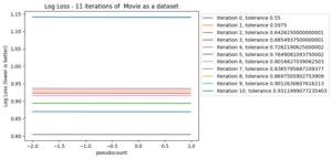
The "movie-as-dataset" predictor

For the "movie-as-a-dataset" predictor, I repeat the process from the matrix multiplication predictor. I chose a few different tolerances, $\sigma =0.95$ and $\sigma =0.99$ and the same ascending and descending tolerances as before, $\sigma _{i}=0.95^{i+1}$ and $\sigma _{i}=1.5-0.95^{i+1}$ for $i=\{0,...,10\}$.

Log loss on 10 iterations of the movie as dataset predictor and tolerance $\sigma =0.99$. The iterations with $\sigma =0.95$ looks the same.

Log loss on 10 iterations of the movie as dataset predictor and an ascending tolerance $\sigma _{i}=0.95^{i+1}$

Log loss on 10 iterations of the movie as dataset predictor and a descending tolerance $\sigma _{i}=1.5-0.95^{i+1}$

Table 1: Minimum Log Loss along iterations of "movie-as-a-dataset" Predictor with different tolerances

Tolerance model	Iteration 0	Iteration 1	Iteration 2	Iteration 3	Iteration 4	Iteration 5	Iteration 6	Iteration 7	Iteration 8	Iteration 9	Iteration 10
$\sigma =0.95$	0.86960	0.86058	0.89726	0.87892	0.90465	0.86701	0.90321	0.69478	0.40414	0.41202	0.39705
$\sigma =0.99$	0.86960	0.86058	0.89726	0.87892	0.90465	0.86701	0.90321	0.69478	0.40414	0.41202	0.39705
$\sigma _{i}=0.95^{i+1}$	0.86947	0.83903	0.80964	0.76027	0.73065	1.83704	1.83704	1.83704	1.83704	1.83704	1.83704
$\sigma _{i}=1.5-0.95^{i+1}$	0.86947	0.85419	0.82624	0.83123	0.87296	0.86393	1.25116	1.71523	1.71523	1.71523	1.71523

Note that the consistent tolerances $\sigma =0.95$ and $\sigma =0.99$ share the same minimums at each iteration. We can observe that in the charts above that a pattern is created (noting that the line colours are different between the charts).

Iterative prediction spreads

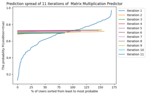
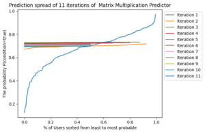
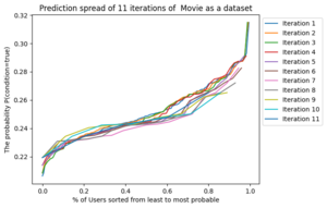
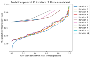
Plotting the probability of passing the given condition and sorting the results from lowest to highest, as well as, expanding the data to overlap as the set size shrinks gives interesting visuals.

For both the matrix multiplication and "movie-as-a-dataset" predictors, looking at the probability distribution of each iteration makes a couple things clear.

Matrix Multiplication Predictor

Prediction spread of matrix multiplication predictor with consistent tolerance $\sigma =0.95$.

Prediction spread of matrix multiplication predictor with consistent tolerance $\sigma =0.99$.

Prediction spread of matrix multiplication predictor with an ascending tolerance $\sigma _{i}=0.95^{i+1}$

Prediction spread of matrix multiplication predictor with a descending tolerance $\sigma _{i}=1.5-0.95^{i+1}$

"Movie-as-a-dataset" Predictor

Prediction spread "movie-as-dataset" predictor with consistent tolerance $\sigma =0.95$.

Prediction spread "movie-as-dataset" predictor with consistent tolerance $\sigma =0.99$.

Prediction spread "movie-as-dataset" predictor with ascending tolerance $\sigma _{i}=0.95^{i+1}$.

Prediction spread "movie-as-dataset" predictor with descending tolerance $\sigma _{i}=1.5-0.95^{i+1}$.

We can see why the matrix multiplication predictor never got to 10 iterations on $\sigma =0.99$. The difference in probabilities is tiny and after 8 iterations it goes down again.

Maximum Probable Difference

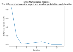
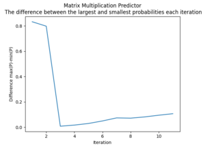
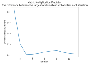
As iterations go on, it's expected that the difference in the highest and lowest probability of a set shrinks. The idea is that these iterations are "pinching" the data towards a uniform distribution - until the last members can be considered their own group. We can also think of the iterations as "shaving off" layers, where each layer does not have to be uniform nor symmetric.

This range of options is something that seems interesting to look at as future work.

Matrix Multiplication Predictor

The maximum prediction difference for the matrix multiplication predictor with $\sigma =0.95$ over multiple iterations.

The maximum prediction difference for the matrix multiplication predictor with $\sigma =0.99$ over multiple iterations.

The maximum prediction difference for the matrix multiplication predictor with $\sigma _{i}=0.95^{i+1}$ over multiple iterations.

The maximum prediction difference for the matrix multiplication predictor with $\sigma _{i}=1.5-0.95^{i+1}$ over multiple iterations.

"Movie-as-a-dataset" Predictor

The maximum prediction difference for the "movies-as-a-dataset" predictor with $\sigma =0.95$ over multiple iterations.

The maximum prediction difference for the "movies-as-a-dataset" predictor with $\sigma =0.99$ over multiple iterations.

The maximum prediction difference for the "movies-as-a-dataset" predictor with $\sigma _{i}=0.95^{i+1}$ over multiple iterations.

The maximum prediction difference for the "movies-as-a-dataset" predictor with $\sigma _{i}=1.5-0.95^{i+1}$ over multiple iterations.

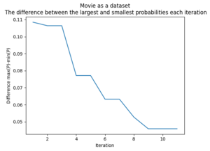
One of the challenges with this approach will be balancing a decreasing difference in probability with the number of iterations. More iterations will provide a larger diversity in the set of values while a smaller difference will make the iteration contain a smaller set.

Conclusion

The iterable prediction reveals some interesting results such as the prediction spread of the "movie-as-a-dataset" predictor with ascending and descending tolerances having some iterations where the minimum probability of the conditional being true is quite high.

It also gives a helpful visualization of how the log loss changes and how certain probability distributions "collapse" as iterations go on and the leftovers become more uniform. This uniformity could be a useful value in deciding the number of iterations and their tolerances.

I believe there is a lot more that can be built off of this. This is only a portion of what I had wanted to achieve, but provides the foundational idea and some insight into how a couple predictors are be affected by being turned into iterable predictors. Future ideas include demonstrating the effects on other predictors, implementing the prediction of ratings with a modified gender domain, and seeing how different datasets would allow for more accurate results.