Course:CPSC522/Density-Based Unsupervised Learning

Density-Based Unsupervised Learning

Density-Based Unsupervised Learning is a kind of unsupervised learning(clustering) method, which is good at finding arbitrarily shaped clusters automatically.

Principal Author: Jiahong Chen

Papers refer to:

1. A Density-Based Algorithm for Discovering Clusters in Large Spatial Databases with Noise, Martin Ester, Hans-Peter Kriegel, Jiirg Sander, Xiaowei Xu.

2. An Efficient Approach to Clustering in Large Multimedia Databases with Noise, Alexander Hinneburg, Daniel A. Keim. (DENCLUE 1.0)

3. DENCLUE 2.0: Fast clustering based on kernel density estimation, Alexander Hinneburg, and Hans-Henning Gabriel

Abstract

Unsupervised learning(clustering) is a computational process to discover clusters in a large databset automatically without the help of prior knowledge to these data, and involves methods at the intersection of artificial intelligence, machine learning, statistics, and database systems.. However, old clustering methods requires much domain knowledge to determine input parameters and do not perform well in finding arbitrarily shaped clusters such as "S" shape and oval clusters. Density-Based Unsupervised Learning is then designed to solve such problems. This page gives a brief introduction to Density-Based unsupervised learning by introducing the motivation of designing such method, presenting two famous Density-Based algorithms and comparing algorithms to exam how new methods outperforms old ones.

Builds on

Density-Based Unsupervised Learning is a computational process, which builds on cluster analysis, unsupervised learning and Data Mining.

Related Pages

Density-Based Unsupervised Learning involves algorithms and methods at the intersection of artificial intelligence, machine learning, statistics, and database systems..

Content

Introduction

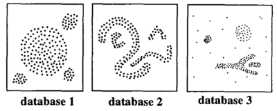
Recently, information explosion has brought numerous data to people, and the type of such data stored in databases are increasingly complex. For easier retrieval, set of numerous data are often clustered in multiple groups to make data object in same group are highly similar, while very different to other data objects in different groups. However, old unsupervised learning methods such as partitioning and hierarchical are only suitable for grouping spherical-shaped clusters. It will be difficult for them to find clusters of arbitrary shape like "S" and oval clusters in Figure 1. Moreover, it will be harder for such method to generate good result if the dimension of the dataset become higher, and noise and outliers are more likely to be included into clusters.

Figure 1: Arbitrary Shaped Cluster

In order to solve such problems, researchers proposed clustering methods based on the density of the data space, dense regions will be separated by sparse regions and group into same cluster according to such separated areas. This is the main thinking of density-based unsupervised learning methods, which solves the problem of old methods cannot find arbitrary shaped cluster well. In the following page, two density-based unsupervised learning methods, DBSCAN(M. Ester et al., 1996) and DENCLUE(A. Hinneburg et al., 1998) will be introduced. Furthermore, comparison between density-based unsupervised learning methods and other old unsupervised learning methods will be presented to tell how density-based unsupervised learning methods is advanced. Also, the superiority of DENCLUE when comparing to DBSCAN will be explained.

DBSCAN: Density-Based Clustering Based on Connected Regions with High Density(M. Ester et al.)

Introduction

The basic idea of DBSCAN is to recognise the clusters that within each cluster it has obvious higher density than outside of the cluster, and we are able to separate different clusters by those low density area. Take Figure 2 for example, we could easily recognise different clusters, noise and outliers. Such process is easy to carry out by human eyes, but hard for computers which has low intelligence. In this way, some definitions to determine high density areas should be made.

Figure 2: DBSCAN Sample database

Definitions

Give a dataset D, the key to decide an data point is inside a dense region or not is to check if it have a high density neighbourhood. In an other words, given a radius $\epsilon$>0, the neighbourhood of those points of inside a dense region should contain at least a minimum number(threshold) of points. The neighbourhood of an point o is the space within a radius $\epsilon$ centred at o, and the distance between two points p and q, which checks if two points are within the radius or not, is determined by distance function, denoted by dist(p,q). In this page, examples are computed with the help of most common distance function, Euclidean distance.

 Definition 1: ($\epsilon$-neghbourhood of a point) The $\epsilon$-neghbourhood of a point p, denoted by $\mathbb {N} _{\epsilon }(p)$, is defined as  $\mathbb {N} _{\epsilon }(p)={q\in D|dist(p,q\leq \epsilon )}$

Meanwhile, after radius $\epsilon$ fixes the neighbourhood size of each point, the density of a neighbourhood can be decided by simply counting the number of points in the neighbour. Another parameter MinPts, which specifies the density threshold of the neighbour, determines a neighbourhood of a point is dense if it contains more than MinPts points. Once we decide a point is in the high density neighbour, we regard it as a core points and then expand it to a larger cluster, with the help of definitions direct density-reachable, density-reachable, density-connected.

 Definition 2: (directly density-reachable) A point p is directly density-reachable from another point q with regard to $\epsilon$ and MinPts if:
 1. p $\in$$N_{\epsilon }(q)$and
 2. $|N_{\epsilon }(q)|$$\geq$MinPts(core point condition)

Obviously, directly density-reachable is symmetric for pair p and q, with the exception that one core point and one border point are involved. In another word, if p is directly density-reachable to q, the directly density-reachable property is not mutual only when q is a border point, who does not have at least MinPts points in its neighbourhood. In general, such point contains significantly less points in its neighbourhood but it should still be include in a cluster(see Figure 3(a)). So we cannot simply set a strict small threshold for MinPts to count in points in a cluster because this will easily confuse cluster points with noise points. Therefore, border points should be better expanded into a cluster by core points. DBSCAN requires that for every point p in a cluster C, there exists a core point q that contains p in its high density neighbourhood.

Figure 3: DBSCAN Border Point

 Definition 3: (density-reachable) A point p is density-reachable from a point q with regard to $\epsilon$ and MinPts if there is a chain of points $p_{1},p_{2},\cdots ,p_{n}$, $p_{1}=q$, $p_{n}=p$ such that $p_{i+1}$is directly density-reachable from $p_{i}$

Note that density-reachable is not an equivalence relation because it is not symmetric. For example, if $p_{1}$ and $p_{n}$ are both core points, they are mutually density reached. However, according to the definition, $p_{n}$ might be border points, which may not be density-reachable to $p_{1},p_{2},\cdots ,p_{n-1}$. In this way, two border points are likely not density reachable form each other because they are both not core points. Therefore, DBSCAN introduced an new concept, density-connected to connect points in same cluster.

 Definition 4: (density-connected) A point p is density-connected to a point q with regard to $\epsilon$ and MinPts if there is a core point o are density-reachable to both p and q with regard to $\epsilon$ and MinPts.

Unlike density-reachable, density-connected is an equivalence relation. It is clear that, for points $p_{1}$, $p_{2}$ and $p_{3}$, if $p_{1}$ and $p_{2}$ are density-connected, and $p_{1}$ and $p_{3}$ are density-connected, $p_{2}$ and $p_{3}$ will also be density-connected.

 Example: To better understand density-reachability and density-connectivity, an example is shown here. As figure 4 shows, left side circles is to indicate density-reachability situation and the right side is for density-connectivity. The $\epsilon$ for this example is the radius of circles and the MinPts is set to 3. 
 For those labeled points, m, p, o, r are core points with regard to $\epsilon$ and MinPts. So, it is clear that m and p are mutually directly density-connected, while m, p is directly density-connected to q but not vice versa. As for the right side, s and r are density-connected with the help of point o. Therefore, s, o, r are all density-connected.

Figure 4: DBSCAN example

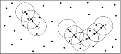
Now, the cluster of DBSCAN could be defined, it is a set of density-connected points and noise points will be allocated to a given set of cluster that not belonging to any other valid clusters.

 Definition 5: (cluster) Given D as a set of data points, a cluster C with regard to $\epsilon$ and MinPts is a non-empty subset of D when:
 1. For any point p and q, if p $\in$ C  is density-reachable from q with regard to $\epsilon$ and MinPts, then q $\in$ C
 2. For any point p, q $\in$ C: p is density-connected to q with regard to $\epsilon$ and MinPts.

 Definition 6: (noise) Let $C_{1},C_{2},\cdots ,C_{k}$ be the clusters of the database D with regard to $\epsilon$ and MinPts. Noise is the set of points in D not belonging to any cluster $C_{i}$.

Algorithm

With all these definitions, we are then able to find DBSCAN clusters. First, all points in the database D are marked as unvisited. Second, algorithm will randomly select a unvisited point p and mark it as visited, then check if this point has at least MinPts points in its $\epsilon$-neighbourhood. If yes, a new cluster C will be created for p, and all the objects in its $\epsilon$-neighbourhood will be add to a candidate set, N. Otherwise, this point will be temporarily marked as noise. Then, for the candidate set N, DBSCAN will add points, which are not belong to other clusters, inside it to same cluster C. When carrying out this process, DBSCAN will mark unvisited points as visited and check its $\epsilon$-neighbourhood. If the $\epsilon$-neighbourhood of these newly added points has at least MinPts points, those points in these $\epsilon$-neighbourhoods will also be added to N. Points will continuing adding objects to C until C cannot expand further, i.e., N is empty. Next, we could start to find next cluster, DBSCAN will randomly choose one unvisited point from rest ones.

The detailed algorithm structure is shown as a persudo below:

 DBSCAN (SetOfPoints, Eps, MinPts)
      //SetOfPoints is UNCLASSIFIED
      ClusterId := nextId(NOISE);
      FOR i FROM 1 TO SetOfPoints.size() DO:
           Point := SetOfPoints.get(i);
           IF Point.CLID = UNCLASSIFIED THEN
               IF ExpandCLuster(SetOfPoints, Point, ClusterId, Eps, MinPts) THEN
                    CLusterId := nextId(ClusterId)

 Boolean ExpandCLuster(SetOfPoints, Point, ClusterId, Eps, MinPts)
     seeds := SetOfPoints.regionQuery(Point, Eps);
     IF seed.size<MinPts Then
         SetOfPoint.changeCLID(Point, Noise);
         RETURN False;
     ELSE
         SetOfPoints.changeCLIDs(seeds, CLID);
         seeds.delete(Point);
         While seeds != Empty Do
              currentP := seeds.first();
              result := SetOfPoints.regionQuery(currentP, Eps);
              IF results.size >= MinPts Then
                  FOR i From 1 TO result.size DO
                       resultP := result.get(i);
                       IF resultP.CLID IN(UNCLASSIFIED, NOISE) THEN
                           IF resultP.CLID = UNCLASSIFIED THEN
                               seeds.append(resultP);
                           SetOfPoints.chengeCLID(resultP, CLID);
              seeds.delete(currentP);
         RETUEN TRUE

DENCLUE(A. Hinneburg et al.)

As the fast technological progress, the amount of data stared in databases increases very fast, and become more and more complex. Old hierarchical clustering methods and density based methods like DBSCAN are no more suitable for the on going task because they are not designed for clustering high-dimensional feature and cannot deal with large amount of noise. And they degenerates rapidly with increasing dimension. Therefore, researchers proposed an new density-based algorithm, DENCLUE(DENsity-based CLUstEring), to solve such problem(A. Hinneburg et al.).The advantages of this new approach are (1) it has a firm mathematical basis, (2) it has good clustering properties in data sets with large amounts of noise, (3) it allows a compact mathematical description of arbitrarily shaped clusters in high-dimensional data sets and (4) it is significantly faster than existing algorithms.

In old density-based methods like DBSCAN and OPTICS, density is calculated by counting the number of objects in a neighbourhood defined by a radius parameter $\epsilon$. Such density is highly sensitive to the radius value. For example, figure 5 shows that the slight change in radius will make a significant change in the point's density.

Figure 5: Radius-Sensitive Density

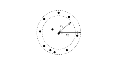
To overcome this problem, kernel density estimation should be applied, which is a non-parametric density estimation approach from statistic. The general idea of kernel density estimation is that we treat an observed object as an indicator of high probability density in the surrounding region. Then the probability density of a point is relating the the distance from itself to the observed objects. Further more, in 2007, A. Hinneburg et al., improved DECLUE to second edition to overcome such shortcoming of old methods. Old methods including DENCLUE 1.0 only use directional information of the gradient, which makes the step size fixed through out the whole hill climbing process. Such problem cause several disadvantages, namely the hill climbing only get close to local maximum but do not converge. And it may iterate too many times because of many unnecessary small steps in the beginning. In this way, DECLUE 2.0 introduced a new hill climbing method for kernel density estimation with Gaussian kernels.

Formally, The kernel density approximation of the probability density function is:

$f(x)={\frac {1}{nh}}\sum _{i=1}^{n}K({\frac {x-x_{i}}{h}}),$

Where $x_{1},x_{2},\cdots ,x_{n}$ be the independent and identically distributed sample of a random variable f, K() is a kernel and h is the bandwidth serving as a smoothing parameter. DENCLUE use Gaussian function with a mean of 0 and a variance of 1 as kernel function K():

$K({\frac {x-x_{i}}{h}})={\frac {1}{\sqrt {2\pi }}}e^{-{\frac {(x-x_{i})^{2}}{2h^{2}}}}.$

Figure 6 shows an example of a set of 2D data chooosing different kernel function, square wave and Gaussian. The left figure is the visualization of the 2D dataset. The middle one is the density result by using square wave as the kernel function, while the right figure is the result of using Gaussian function.

Figure 6: Examples Of Densty Functions

DENCLUE uses a Gaussian kernel to estimate the density based on the given set of objects to be clustered.A point $x^{*}$ is called a density attractor if it is a local maximum of the estimated density function. So, DENCLUE uses a threshold $\xi$ to avoid trivial local maximum points. And it only count those density attractors $x^{*}$if $f(x^{*})\geq \xi$ as the center-defined clusters.

Data points are allocated to different clusters with the help of density attractors using a step-wise hill-climbing procedure. For an point x, the hill-climbing procedure starts form x and is guided by the gradient of the estimated density function. These density attractors are computed as:

$x_{j+1}=x^{j}+\delta {\frac {\nabla f(x^{j})}{|\nabla f(x^{j})|}}$

where $x^{0}=x$ and $\delta$ is the parameter for controlling the speed of converge, and $\nabla f(x)$ is the gradient of density function $f(x)$

Such hill-climbing procedure stops at step k, where k>0 and $f(x*{k+1}<f()x^{k})$, then assigns x to the density attractor $x^{*}=x^{k}$. Moreover, point x is the outlier or noise if it converges in such process to a local maximum $x^{*}$ with $f(x^{*})<\xi$.

A cluster in DENCLUE is a set of density attractors X and a set of input points C, where each point in data set C will be assigned to a density attractor $x^{*}$ in X. Besides, there exists a path between every pair of density attractors where the density is more then $\xi$. Figure 7 indicates how DECLUE find arbitrary-shaped clusters using different $\xi$. By using multiple density attractors, $x^{*}$, who connected by paths, the algorithm will then able to find clusters of arbitrary shape.

Figure 1: Examples of Arbitrary-Shaped Cluster for different parameter

Comparison

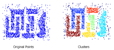
In this section, the advantage of DBSCAN when comparing to old methods will firstly be presented. As figure 8 shows, DBSCAN are able to find arbitrary shaped clusters. It is more useful when comparing to old methods, like K-means which can only find round-shaped clusters.

Figure 8: DBSCAN Advantage

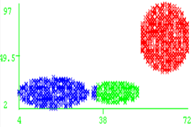
However, it still has same shortcomings, we have to manually set the threshold for DBSCAN, which results in it sometimes cannot perform well if parameters does not suitable for the dataset. Moreover, DBSCAN might not perform well if clusters are close and density varies. Figure 9 is an example indicates the situation that two clusters are close and cause DBSCAN did not make the correct grouping. As we can see, blue cluster and green cluster are too close and some of points are not correctly allocated.

Figure 9: DBSCAN Disadvantage

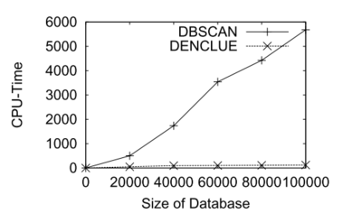
Next, the advantage of DECCLUE will be examined. Authors tested the algorithm using real multimedia datasets including CAD and molecular biology application. They transformed the polygonal CAD data into 11-dimensional feature vectors with the help of Fourier transformation. The number of points in the dataset varies from 20000 to 100000. The comparison result of computing time with DBSCAN is shown as figure 10. As we can see, DENCLUE is much faster than DBSCAN in this high dimensional dataset.

Figure 10: Comparison

Moreover, effectiveness of DENCLUE could be examined. The algorithm is applied to an application in the area of molecular biology. The data used for the test comes from a complex simulation of a very small but flexible peptide. And it is generated by the simulation which describes the conformation of the peptide as a 19-dimensional point in the dihedral angle space with around 10000 points. Since there are large amount of high-dimensional data, it is difficult to find the preferred conformations of the molecule. Furthermore, the flexibility of the peptides is responsible for the fact that the peptide has many intermediate non-stable conformations which causes the data to contain large amounts of noise, more than 50 percent.

Figure 11: Folded Conformation of the Peptide

Figure 11 indicates the most important conformations found by DENCLUE(figure 11a). Such conformations are corresponding to the largest clusters of conformations in the 19-dimensional dihedral angle space, which is not able to found by DEBSCAN.

To Add

Put links and content here to be added. This does not need to be organized, and will not be graded as part of the page. If you find something that might be useful for a page, feel free to put it here.