Course:CPSC522/Action Selection for MDPs

Action Selection for MDPs

This page explores two approaches for action selection in Markov Decision Problems

Principal Author: Bronson Bouchard
Collaborators:

Abstract

Action selection for large state-space Markov Decision Problems is done by intelligently computing the optimal policy then taking the action that will result in the best state. A recent popular method is applying Upper Confidence Bounds to Trees (UCT). This page will briefly describe UCT and explore two alternatives to UCT for action selection, Anytime AO* and MAXQ-OP.
The papers that will be covered are:
Bonet, Blai, and Hector Geffner. "Action Selection for MDPs: Anytime AO* Versus UCT." AAAI. 2012.
Bai, Aijun, Feng Wu, and Xiaoping Chen. "Online planning for large markov decision processes with hierarchical decomposition." ACM Transactions on Intelligent Systems and Technology (TIST) 6.4 (2015): 45.

Builds on

The action selection discussed is for an agent in a Markov Decision Process.

Introduction

Markov Decision Processes (MDPs) are widely used in modeling decision making tasks. MDPs are applied to decision making in games, in navigation problems, and in many other domains. There have been many different approaches to finding an optimal policy in MDPs, each method has varying effectiveness depending on the problem. In large state-spaces it is not possible to explore every action fully and as such the choice of nodes to expand is important. MDPs can have many different properties, the specific type discussed in this page are fully observable infinite horizon MDPs. Bonet and Geffner take the approach of using a heuristic search for finite MDPs applied to an infinite horizon and compare against the UCT algorithm.

Action Selection for MDPs: Anytime AO* Versus UCT

MDP Notation

An MDP consists of:

• A set of states $S$
• A set of actions $A(s)$ that can be applied to each state
• A Transition Probability $Pa(s'|s)$ of moving from a state $s$ to a new state $s'$

When taking an action there is some reward associated as a result $r(a,s)$ or a cost $c(a,s)$. A discount factor a discount factor $\gamma$ can be used to weight immediate actions and future actions where $0<\gamma <1$. The solution to a MDP is a policy $\pi$ that selects an action in each state.

Anytime AO* Algorithm

AO* is an algorithm that can be used to search in an AND-OR graph. An anytime algorithm is an algorithm that can be terminated at any time and will return some answer and the answers returned improve as a function of time. A finite-horizon MDP defines an implicit AND/OR graph (AND nodes requiring all children be evaluated, OR nodes only requiring one) which can be solved by AO*. The graph that AO* is run on is modeled as:

• Root node (s0, H), s0 is inital state, H is the horizon
• Internal nodes (a, s, d) where a is an action to be performed on the state s and d is the remaining depth in the horizon
• Terminal nodes (s,d), d = 0
• The child of an internal node is (s',d-1), where s' is the state resulting from the action selected

AO* uses an admissible heuristic to search over the graph, the heuristic is a function that provides an estimated reward/cost that will be the result of taking an action and transitioning to the next state. An admissible heuristic is a heuristic that does not overestimate the reward. This heuristic intelligently orders nodes that will be expanded and expands the highest reward nodes, applying their corresponding actions to the states. The result of the search is a path including every child of an AND node and the optimal choice from an OR node. The search is performed by keeping two graphs, an explicit graph G and a best partial solution G* where the explicit graph is the expansion of the implicit graph. Nodes in the best-partial graph which have children (a,s,d) are iteratively explicated and put in the explicit graph until only terminal nodes exist. As each node is explicated, the value of the node is set to the heuristic value and the best partial solution is updated. Anytime AO* (abbreviated to AOT) extends AO* by allowing non-admissible heuristics and randomly sampled heuristics as a base policy. Allowing non-admissible heuristics can greatly increase the flexibility by allowing more options for heuristics and can significantly reduce execution time. This is is done by incorporating a probability that the node to explicate is selected from the best-partial graph or from the rest of the graph, this includes some exploration as a non-admissible heuristic may guide the search incorrectly if just exploited. Random heuristics are included by sampling of the heuristic function until a node is fully expanded, each sample of the heuristic is averaged with the previous samples.

The Pseudo code for Anytime AO* is as follows

Anytime AO*: G is explicit graph, initially empty; h is heuristic function; p, 0 ≤ p ≤ 1
1. Insert node (s, H) in G where s is the initial state
2. Initialize V (s, H) := h(s, H)
3. Initialize best partial graph to G
    Loop
	 4.1. Choose IN with probability 1 − p, else Choose OUT:
		• IN: Select non-terminal tip node (s, d) from explicit graph G that is IN the best partial graph
		• OUT: Select non-terminal tip node (s, d) from explicit graph G that is NOT in the best partial graph
	4.2. If there is no node (s, d) satisfying the choice condition, make the other choice. If there is no node satisfying either choice condition, Exit the loop
       5. Expand node (s, d): 
               for each a ∈ A(s)
                 add node (a, s, d) as child of (s, d)
               for each s' with Pa(s'|s) > 0
                  add node (s', d − 1) as child of (a, s, d)
               Initialize values V (s', d − 1) for new nodes (s', d − 1) as 0 if d − 1 = 0, or h(s', d − 1) otherwise.
        6. Update ancestors AND and OR nodes of (s, d) in G, bottom-up as: Q(a, s, d) := c(a, s) + γΣs' Pa(s'|s)V (s', d − 1), V (s, d) := mina∈A(s)Q(a, s, d)
        7. Mark best action in ancestor OR-nodes (s, d) to any action a such that V (s, d) = Q(a, s, d), maintaining marked action if still best
        8. Recompute best partial graph by following marked actions

UCT Algorithm

The UCT algorithm incrementally expands a graph by selecting nodes based off of stochastic simulations. The search is guided by a search constant C and counters for how many simulations have been done on each node, and which actions were chosen, which make up the bonus term. The bonus term serves to minimize the regret of choosing actions and balances exploration with exploitation as the other term would only exploit the known structure in the search. The discounted reward is sampled by simulating the base policy from a given state to a depth of d which is then propagated up by Monte-Carlo backups.

UCT pesudo code:

UCT(s, d): G is explicit graph, initially empty; 
π is base policy; C is exploration constant,
N(s, d) is a counter for how many simulations passed through a node,
N(a,s,d) is the number of times action a was selected a the node
1. If d = 0 or s is terminal, Return 0
2. If node (s, d) is not in explicit graph G, then
	Add node (s, d) to explicit graph G
	Initialize N(s, d) := 0 and N(a, s, d) := 0 for all a ∈ A(s)
	Initialize Q(a, s, d) := 0 for all a ∈ A(s)
	Obtain sampled accumulated discounted reward r(π, s, d) by simulating base policy π for d steps starting at s
	Return r(π, s, d)
3. If node (s, d) is in explicit graph G,
	Let Bonus(a) = $C{\sqrt {2logN(s,d)/N(a,s,d)}}$ if N(a, s, d) > 0, else ∞, for each a ∈ A(s)
	Select action a = argmaxa∈A(s)[Q(a, s, d) + Bonus(a)]
	Sample state s0 with probability Pa(s0|s)
	Let nv = r(s, a) + γUCT(s0, d − 1)
	Increment N(s, d) and N(a, s, d)
       Set Q(a, s, d) := Q(a, s, d) + [nv − Q(a, s, d)]/N(a, s, d)
       Return nv

Evaluation
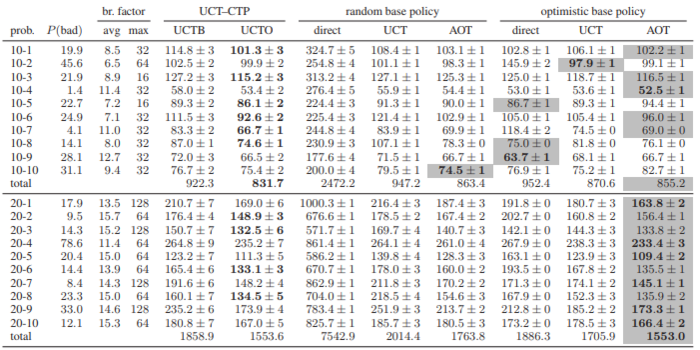
The authors compared their contribution of AOT against UCT by testing both algorithms in three problems: The Canadian Traveller Problem, a sailing problem similar to the original UCT paper, and a race track problem. In the Canadian Traveller Problem AOT achieved lower cost results in less execution time. In the sailing problem and the race track problem both algorithms performed comparably.

Problem instances with 10 and 20 nodes, P(bad) is the probability the instance is not solvable. UCTB and UCTO are two domain-dependent UCT implementations Boldface figures are best in whole table; gray cells show best among domain-independent implementations

AOT performs only slightly better than UCT but it provides a different approach than UCT to the problem.

Online planning for large markov decision processes with hierarchical decomposition

This paper is also focused on MDPs with a large state-space that instead uses MAXQ hierarchical decomposition in the online setting, attempting to exploit an underlying hierarchical structure of the problem. The approach taken is to split the MDP into sub tasks and perform online planning while exploiting the hierarchical structure. MAXQ task hierarchies are used instead of recording complete policies for each subtask, the task hierarchy includes active states, goal states, and local-reward functions for all sub tasks. The local-reward functions are programmed in and are optional.

MAXQ-OP Hierarchical Decomposition

MAXQ Hierarchical Decomposition defines a set of sub-MDPs arranged over a hierarchy, formed as a directed acyclic graph. Each sub task has termination predicate which is used to separate active states from terminal states as well as a set of actions and an optional local reward function. The hierarchical decomposition can be done to any input MDP but the decomposed task-graph must be supplied.

• Given an MDP $M$, a set of decomposed MDPs is $\{M_{0},M_{1},...,M_{n}\}$
• $M_{0}$ is the root subtask that solves $M$
• a hierarchical policy is a set of policies for each subtask $\pi =\{\pi _{0},\pi _{1},...,\pi _{n}\}$ where $\pi _{i}:S_{i}\rightarrow A_{i}$
• $V^{\pi }(i,s)$ is projected value function which is equal to the cumulative reward following a hierarchical policy $\pi$.
• $Q^{\pi }(i,s,a)=V^{\pi }(a,s)+C^{\pi }(i,s,a)$ the value functions of a hierarchical policy
• $C^{\pi }(i,s,a)$ is the completion function which is the expected cumulative reward after finishing subtask _a and before M_i
• The optimal policy can be found by computing the optimal projected value Q^∗(i, s, a) = V^*(a, s) + C^∗(i, s, a)
• $\pi _{i}^{*}(s)=argmax_{a\in A_{i}}Q^{*}(i,a,s)$ is the optimal policy for a subtask

The online planning is done by approximating the optimal policy $Q^{*}(i,s,a)$. the completion function is too expensive to compute so it is estimated.

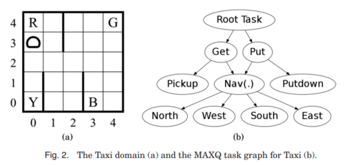
An example task-graph which results from decomposing the MDP into a hierarchy of sub tasks of the taxi problem. (Fig. 2)
The Taxi domain is a problem is a grid world containing a taxi, a passenger, and four designated pickup and drop off locations. The taxi starts in a random location and a passenger starts at one of the four locations and has a desired destination. The taxi's job is to pick up the passenger and drop them off at the desired destination, moving in the four cardinal directions. The example is fully explained and MAXQ applied to in Dietterich, 2000.

The pseudo code is as follows:

OnlinePlanning()
Input: an MDP model with its MAXQ hierarchical structure
Output: the accumulated reward r after reaching a goal 
1. Let r ← 0;
2. Let s ← GetInitState();
3. Let root task← 0;
4. Let depth array← [0, 0, . . . , 0];
5. while s ∉ G0 do
6. 	(v, ap) ← EvaluateStateInSubtask(root task, s, depth array);
7. 	r ←r+ ExecuteAction(ap, s);
8.	s ← GetNextState();
9. return r;

OnlinePlanning() is the main function of the algorithm, looping until a goal state is reached. Each state is initialized by the function GetInitState and the loop iterates through states by the function GetNextState(). The function EvaluateStateInSubtask does a depth-first search returning the best action for the current state.

EvaluateStateInSubtask(i, s, d)
Input: subtask Mi , state s and depth array d
Output: (V∗(i, s), a primitive action ap*)

1. if Mi is primitive then return (R(s,Mi ),Mi);
2. else if s ∉ Si and s ∉ Gi then return (−∞, nil);
3. else if s ∈ Gi then return (0, nil);
4. else if d[i] ≥ D[i] then return (HeuristicValue(i, s), nil);
5. else
6. 	Let (v∗, a∗p) ← (−∞, nil);
7. 	for Mk ∈ Subtasks(Mi) do
8.		 if Mk is primitive or s ∉ Gk then
9. 			Let (v, ap) ← EvaluateStateInSubtask(k, s, d);
10. 			v ← v+ EvaluateCompletionInSubtask(i, s, k, d);
11. 			if v > v∗ then (v∗ , ap* ) ← (v, ap);
12; return (v∗, a*p);

The EvaluateStateInSubtask is a recursive function that builds a search tree starting from the state s and ending at a goal state. The search tree is an AND-OR graph as in the previous paper which is searched by a best-first search until the depth limit d. With the task hierarchy supplied this is the portion of the code that evaluates each subtask M_i, estimates the completion function, and selects the subtask with the highest value.

EvaluateCompletionInSubtask(i, s, a, d)
Input: subtask Mi , state s, action Ma and depth array d
Output: estimated C∗(i, s, a)
1. Let Gs,a ← {s' | s' ∼ Pt(s' | s, a)};
2. Let v ← 0;
3. for s' ∈ Gs,a do
4. 	d' ← d;
5. 	d'[i] ← d'[i] + 1;
6. 	v ← v+ EvaluateStateInSubtask(i, s', d');
7. v ← v/|Gs,a| ;
8. return v;

EvaluateCompletionInSubtask begins another recursion to estimate the completion function. The termination conditions for all subtasks must be specified before starting. The state that is reached is an end state, whether it is a goal state or just a termination point. The returned value is the estimated value of the action.

NextAction(i, s)
Input: subtask index i and state s
Output: selected action a∗
1. if SearchStopped(i, s) then return nil;
2. else
3. Let $a^{*}\leftarrow argmax_{a\in A_{i}}H_{i}[s,a]+c{\sqrt {lnN_{i}[s]/N_{i}[s,a]}};$
4. Ni [s] ← Ni[s] + 1;
5. Ni [s, a∗] ← Ni [s, a∗] + 1;
6. return a∗;

The NextAction function finds the best estimated action to evaluate to direct and speed up the search. The method is subtask specific so different heuristics can be used for each subtasks. The heuristic value H_i is combined with with the same upper confidence bound (UCB) algorithm as used in UCT. Alternatively the paper suggests that the heuristic value can be updated by interacting and learnin with the environment, the function H_i[s, a] ← (1 − α)H_i[s, a] + αQ(i, s, a) is used from reinforcement learning.NextAction also calls the SearchStopped function which determines if the search should stop based on a value threshold or other conditions.

Evaluation
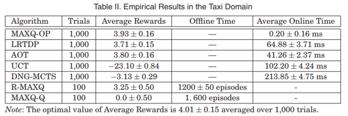
MAXQ-OP was tested against AOT and UCT in a Taxi problem, in which it performed vastly better than AOT and UCT. The paper also examines the application of MAXQ-OP to a 2D soccer (RoboCup 2D) but the taxi results are easier to examine.

The incremental improvement by taking a different approach and including a hierarchy of sub tasks, even if it is required to be programmed, allows MAXQ-OP to achieve better results than ACT which also achieved better results than UCT. The biggest limitation is that the hierarchy has to be supplied, although the authors note it is a research interest to learn the hierarchies instead of supplying them. The performance comparison is not completely fair as the MAXQ-OP implementation incorporates domain knowledge to the search. A future implementation that learned the hierarchy online as well would be a fair comparison but it would be at a cost of performance and quality. The contribution of the second paper is the online MAXQ hierarchical decomposition and the improvements it makes.

Annotated Bibliography

<references>