Course:ASTR508/Notes
Basic Stars, Basic MESA
Reading Assignment
Chapter 1 of Stellar-Astrophysics Notes
Observations of Stars
How to get MESA?
- Download the MESASDK from http://www.astro.wisc.edu/~townsend/static.php?ref=mesasdk and unpack
- Download the recent MESA source by following the instructions at http://mesa.sourceforge.net
- Create your setup.sh script to setup the environment variables for MESA and the MESASDK
- Run the setup.sh script
- Go to the MESA directory and run "./install"
- Get more help at http://mesastar.org/
- If you want to install ctioga2 with your MESASDK, follow my instructions at Ctioga2.
You can also use MESA-Web until you get your own copy working or Cocalc. If you have trouble installing your copy, please try
What does MESA do?
MESA Inlists:
- sample_zams
- create_zams
Assignment
Part 1
Using the estimate of the central temperature of the Sun that I derived in class and the equation for radiative energy transport, estimate the luminosity of the Sun if the opacity is given by electron scattering 0.4 cm2g-1 or by free-free opacity using the mean density and the central temperature of the Sun. Here is the formula for the absorption coefficient in c.g.s. units and its relationship to the free-free opacity :
Take . and are the number densities of electrons and ions respectively. is the atomic number and is the Rosseland mean Gaunt factor.
Part 2
Complete the MESA exercises at the end of chapter one of Stellar Astrophysics .
The easiest way to get the code for the exercises is to download the repository on GitHub at [1].
Also please download [2] to help you get started with MESA>
Equations of Stellar Structure
Reading Assignment
Chapter 2 of Stellar-Astrophysics Notes
Equilibria of Stars
- Hydrostatic
- Thermal
- Nuclear
Hydrostatic Equilibrium
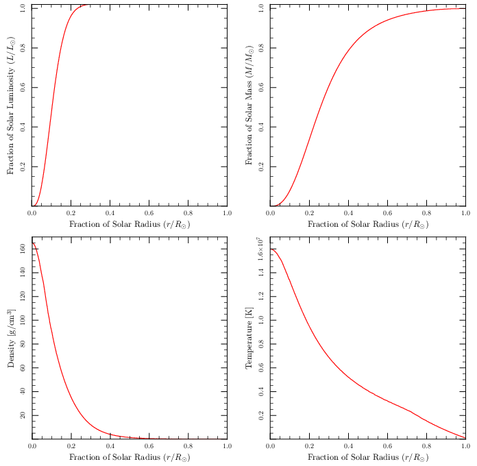
The outward force due to the pressure gradient within the star is exactly balanced by the inward force due to gravity.
- ,
where is the cumulative mass inside the shell at and G is the gravitational constant. The cumulative mass increases with radius according to the mass continuity equation:
Integrating the mass continuity equation from the star center () to the radius of the star () yields the total mass of the star.
Energy Generation
Considering the energy leaving the spherical shell yields the energy equation:
- ,
where is the luminosity produced in the form of neutrinos (which usually escape the star without interacting with ordinary matter) per unit mass. Outside the core of the star, where nuclear reactions occur, no energy is generated, so the luminosity is constant.
Energy Transport
The energy transport equation takes differing forms depending upon the mode of energy transport. For conductive luminosity transport (appropriate for a white dwarf), the energy equation is
where k is the thermal conductivity.
In the case of radiative energy transport, appropriate for the inner portion of a solar mass main sequence star and the outer envelope of a massive main sequence star,
where is the opacity of the matter, is the Stefan-Boltzmann constant, and the Boltzmann constant is set to one.
Convection
Reading Assignment
Chapter 3 of Stellar-Astrophysics Notes
Section 4.3 of Collins
In class we discussed convection using the mixing length theory. One can get similar results without any free parameter according to this recent paper, http://arxiv.org/pdf/1403.6122.pdf !!!
Polytropes
Reading Assignment
Chapter 4 of Stellar-Astrophysics Notes
What are polytropes?
They are a simple model for a star where the pressure is proportional to some power of the density:
Why did we use such an odd exponent? Let's look at the equations of hydrostatic equilibrium and gravity
and we can combine these
Now let's define some dimensionless quantities
where
And now we have a dimensionless equation of the hydrostatic equilibrium with gravity
as known as the Lane-Emden equation. We have to solve this with two conditions at : , so for each value of there is a single solution that we can scale to the size of the star that we are interested in. The solution is only valid where so the surface of the star lies where vanishes, called . There are three closed-form solutions.
and
What do these three solutions mean physically?
Assignment
Calculate the function for various values of between 0 and 5. Some important ones in addition to the ones here are and .
Pre-Main Sequence Evolution
Reading Assignment
Chapter 9 of Stellar-Astrophysics Notes
Star Formation
How long does star formation take?
Jean's Instablity
Stages of a protostar:
- Molecular Cloud
- Spherical accretion
- Disk accretion - T Tauri Star
- Commencement of nuclear burning - building a radiative core
- Main sequence star
Fully Convective Stars and the Hayashi Track
What happens once the bulk of the accretion has ceased and the protostar is no longer rotating quickly?
- Energy is supplied by gravitational contraction.
- The power is limited by how fast the energy can get out of the star:
- The temperature is low so the radiative opacity is high. If the temperature gradient exceeds the adiabatic gradient, convection will start.
- Convection cannot extend all the way to the surface because within a photon mean-free path of the surface, the energy will be carried by radiation and the temperature gradient will drop.
Hayashi Track
Henyey Track
As the star contracts, the centre eventually may get so hot that the radiative opacity is sufficiently small that radiation can carry the energy in the core. A central radiative zone forms.
Low Temperature Opacities
Assignment
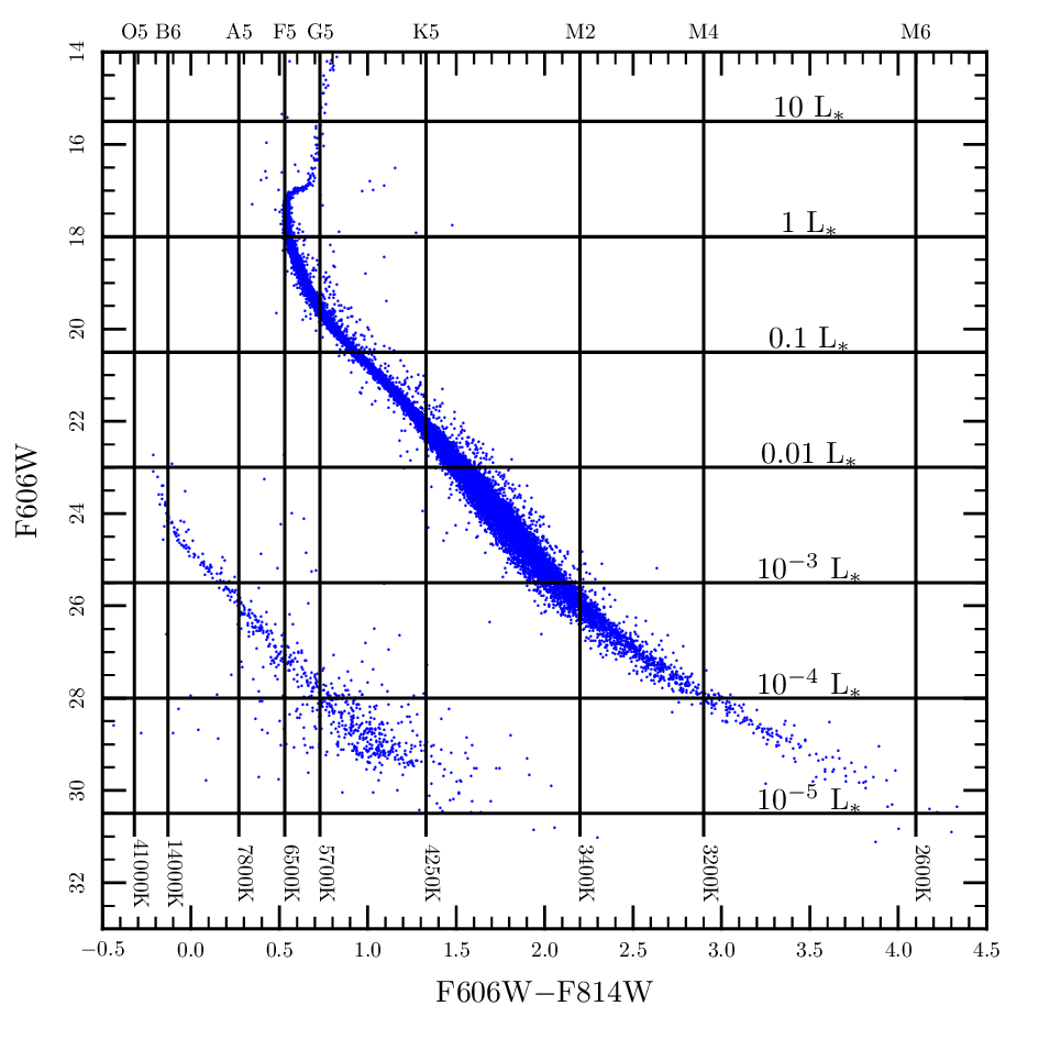
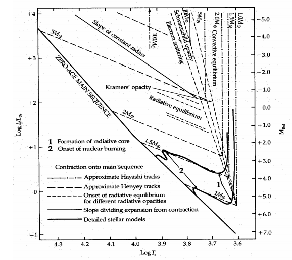
Use the create_zams inlist to make a zero age main sequence for 47 Tucanae. In the process you will run a series of stars through the pre-main sequence for the 47 Tuc metallicity. From these models plot the protostars on a theoretical ( vs ) and observational H-R diagram ( vs ) for several masses: 0.2, 0.5, 0.7, 1, 2, 5, 8, 15 solar masses. How long do protostars of different masses take to reach the main sequence?
Using the output of the MESA runs, indicate the following on your H-R diagrams:
- the time to reach a given position along the track
- the onset of nuclear burning (say when the nuclear luminosity is one tenth of the ZAMS luminosity)
- the formation of the radiative core (how can you figure this out?).
How does the shape of the track of a low mass star differ from a higher mass star? At what mass is the transition? What does this mean?
Nuclear Physics
Reading Assignment
Chapter 10 of Stellar-Astrophysics Notes
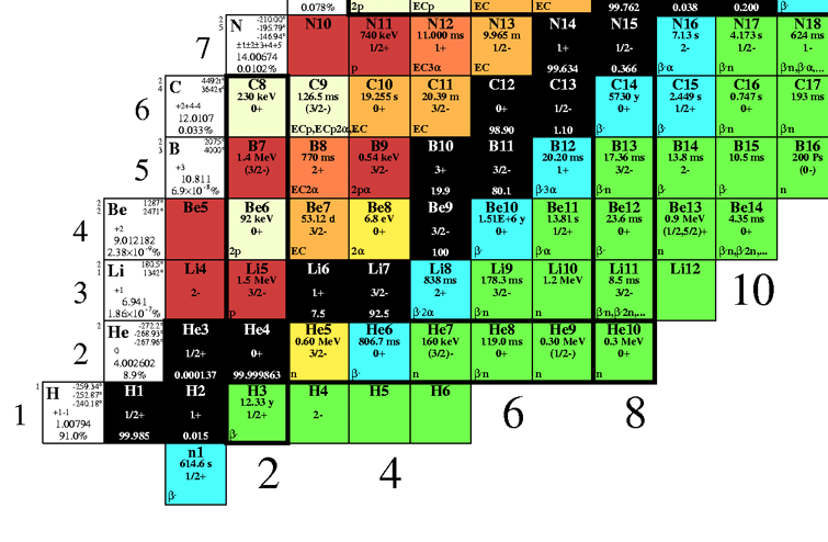
Nuclear Reactions
element Z A M/mu element Z A M/mu  element Z A M/mu
  n 0 1 1.008665   C 6 12 12.000000    Ne 10 20 19.992441
  H 1 1 1.007825     6 13 13.003354    Mg 12 24 23.985043
    1 2 2.014101   N 7 13 13.005738    Si 14 28 27.976930
 He 2 3 3.016029     7 14 14.003074    Fe 26 56 55.934940
    2 4 4.002603     7 15 15.000108    Ni 28 56 55.942139
 Li 3 6 6.015124   O 8 15 15.003070
    3 7 7.016003     8 16 15.994915
 Be 4 7 7.016928     8 17 16.999133
    4 8 8.005308     8 18 17.999160
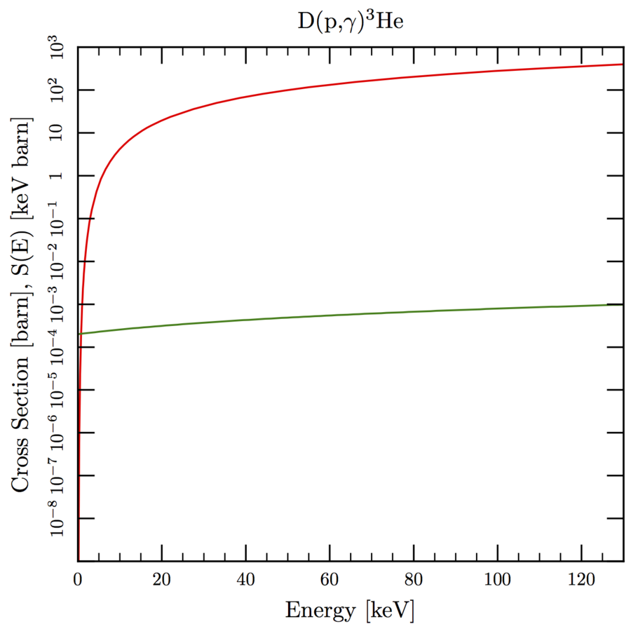
Deuterium
Lithium
Proton-Proton Cycle
Thinking about weak interactions
CNO Cycle
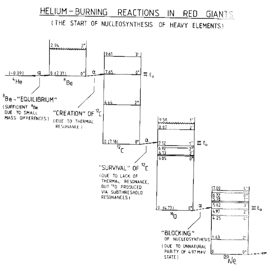
Helium Burning
Nuclear Reaction Rates
Summary
or
 Proton-Proton             CNO Cycle            Triple Alpha
--------------          --------------        --------------
 T6    e0       nu         e0     nu         T8    e0      nu
------------------------------------------------------------------
 10  0.07     4.60        3e-4      22.9    0.8   2e-12    49
 20  1        3.54      4.5e02      18      1.0   4e-8     41
 40  9        2.72        3e07      14.1    2.0   15       19
 80 43        2.08        2e11      11.1    3.0   6e3      12
100   -        -          2e12      10.2    4.0   1e5       7.9
Advanced Nuclear Reactions
Carbon Burning
Neon Burning
Oxygen Burning
Silicon Burning
The Evolution of a Low-Mass Star
Reading Assignment
Chapter 11 of Stellar-Astrophysics Notes
Homology
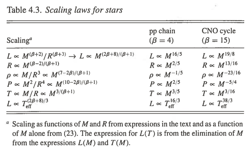
Often in stellar structure one process dominates in a particular region of the star or possibly in the entire star. Furthermore, the form of the equations like the ones above may be multiplicative in nature which can allow us to find scaling relations between the star's mass and its other properties. Let us write
and write the various other quantities as a function of scaled by the total mass to various powers. We have
To make further progress let's write all of the stellar structure equations in terms of the enclosed mass
and substitute the scaling relations
This yields a relationship between the various exponents, . Let's look at the next equation. This has on the right-hand side, so we need a relationship between and the other quantities. This is called the equation of state
For an ideal gas . For a degenerate gas (non-relativistic), and . For a neutron star stuff and . We will leave this quantities open for now, so we have
so
Temperature-Independent Equations of State
If the equation of state does not depend on temperature (), these two equations are sufficient to figure things out. The energy generation and the energy transport equations are important to see how the star shines but not for the structure of the star. We have
so
We can see a couple of interesting things immediately. First for stars get bigger as they get more massive and for more massive stars are smaller in radius. Of course, these equations can apply to any self-gravitating object that ends up spherical and where energy generation doesn't play a role in the structure. For example the radii of objects more massive than Jupiter up until nuclear burning starts are all quite similar, so for these objects. This is thought to be also the case for neutron stars.
The second interesting value of is for which both and diverge. This indicates that the mass for has a fixed value that doesn't depend on the central pressure or the radius of the star, rather it depends on the constant that we defined earlier. Relativistic degenerate electrons have yielding the Chandrasekhar limit for white dwarfs. On the other hand, convective regions also have so the mass of such a region does not depend on its radius but rather on the specific entropy of the fluid which in this case sets --- this limit applies for low-mass stars which are fully convective.
The limit can also be used to understand the most massive stars where radiation pressure dominates. Let us suppose that the pressure due to material is some fraction of the total pressure, so
and
so
and the total pressure is
and .
We know that the pressure within a star must increase as the mass increases, so we find that as the star gets more massive and radiation pressure dominates more and more.
A third interesting limit is a constant density object like a rocky planet (approximately). Here so we have and the radius increases as the cube root of the mass (which makes sense) and the pressure increases as mass to the two-thirds power.
Temperature-Dependent Equations of State
To make further progress (and to have stars that shine) we will have to tackle the other equations of stellar structure. And these require us to define some more constitutive relations. We have the energy generation equation
where we have used the equation of state to eliminate the density from the equation.
For many energy generation processes is large and .
so
We get the following relationships between the exponent of :
and the solutions
where
These are completely general and completely useless. Let's look at thermal pressure from ions () and free-free opacity (, ). Furthermore let's focus on hydrogen burning with . We are left with
For nuclear energy generation processes is large so if we take the limit of we have
As the mass increases the typical density decreases, so eventually free-free opacity is less than electron scattering opacity with and
The luminosity dependence on mass is somewhat more relaxed. Finally at the highest mass stars, the pressure is also dominated by the radiation so additionally we have and and
These relationships reflect the observed mass-luminosity for stars more massive than about half of the mass of the Sun. Less massive stars are fully convective and our analysis did not include convection at all so it cannot apply to these stars.
MESA
MESA Inlists:
- 1M_pre_ms_to_wd (long test)
- solar_calibration
- solar
Stellar Structure of Low-Mass Stars
Less than 0.5
0.5-2
2-8
Assignment
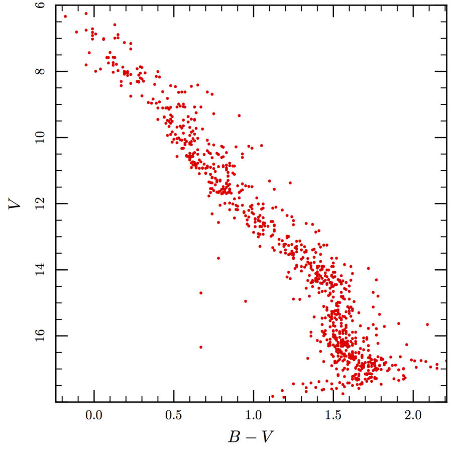
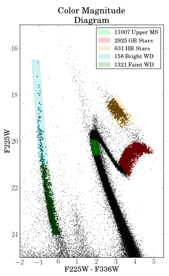
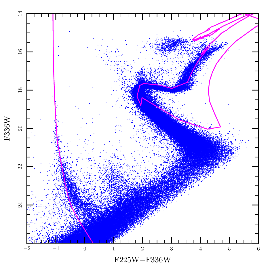
- Using sample_zams as a starting point, generate a CMD in MV vs B-V for a solar metallicity ZAMS and for the metallicity of 47 Tuc (create_zams). If you assume that stars stay the same colour and luminosity on the MS (not strictly true), what does the CMD look like at an age of 10 Myr, 100 Myr, 1 Gyr and 10 Gyr? Using your solar metallcity ZAMS at 100 Myr figure out the distance to the Pleiades and at 10 Gyr for 47 Tuc. You will have to edit the specification file. Use the value of log(tnuc) to estimate which stars are alive after a given time. That is, for 1 Gyr only plot stars with log(tnuc)>9.
For the 47 Tuc model with (create_zams) you will have to remove the line from run_star_extras.f that gets it to stop (look in the docs directory for a hint) and put a control in run_star.extras.f to get it to stop at the end of H-burning, say when the central hydrogen fraction is less than one percent. You can use the star pointer variable: s % center_h1. Make it like the code that you just deleted. The routines create_zams and sample_zams do not make files in the LOG directory, so you will use the final console output to get the data that you need.
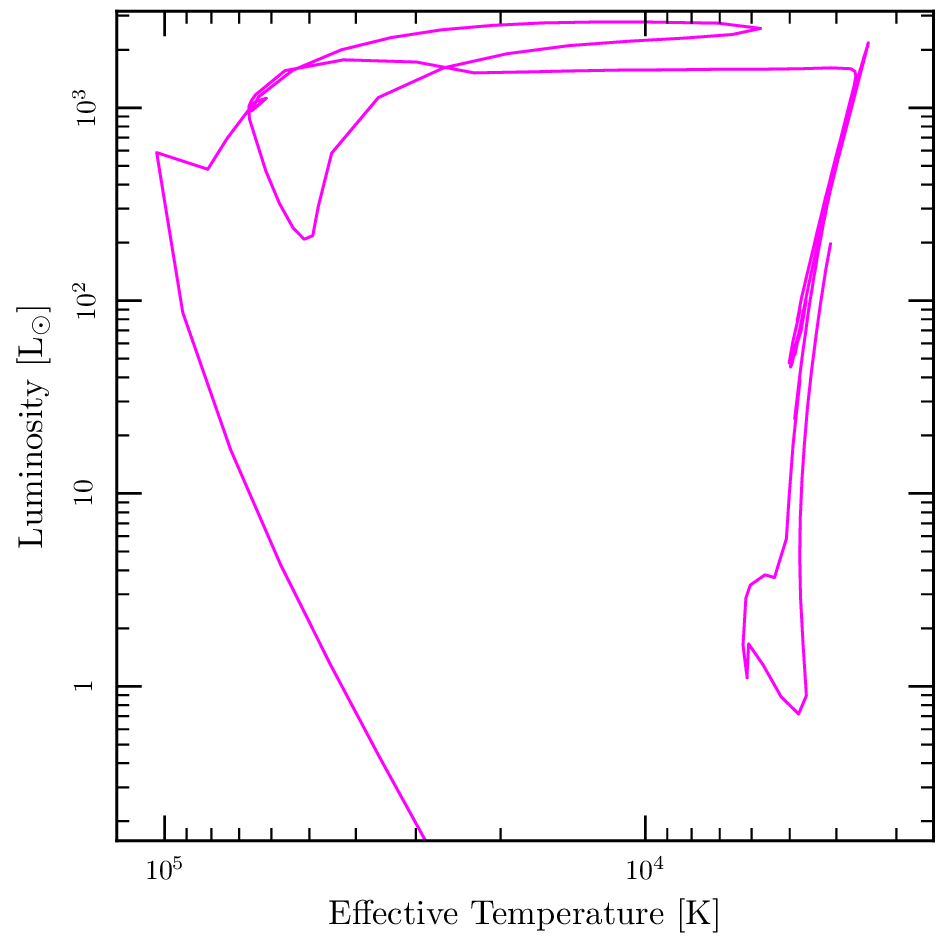
- Generate a CMD for a solar mass star through its entire lifetime (here both L vs Teff and MV vs B-V). Divide the star's history into various stages by looking at the external observables as a function of time. What is going on inside the star during each of these stages? Start with the 1M_pre_ms_to_wd inlist.
You will find the table below useful to convert luminosity and effective temperature to colour.
# SpTyp  MV   BC   MBol   B-V   L/Lsun    Teff  Mass
#  1     2    3     4      5      6        7      8
  M6  16.5   4.3 12.20  1.7  1.0568e-03   2600  0.17
  M4  12.7   2.7 10.00  1.6  8.0168e-03   3200  0.25
  M2  11.2   1.7  9.50  1.5  1.2706e-02   3400  0.3
  M0   8.9   1.2  7.70  1.41 6.6681e-02   3800  0.35
  K7   8.3   1.0  7.30  1.32 9.6383e-02   4000  0.47
  K5   7.5   0.6  6.90  1.08 1.3932e-01   4350  0.69
  K0   5.9   0.4  5.50  0.84 5.0582e-01   5250  0.78
  G5  4.93   0.2  4.73  0.69 1.0280e+00   5700  0.93
 Sun  4.83  0.07  4.76  0.65 1.0000e+00   5780  1
  G0   4.2   0.2  4.00  0.59 2.0137e+00   6000  1.10
  F5   3.3   0.1  3.20  0.41 4.2073e+00   6500  1.3
  F0   2.4   0.1  2.30  0.32 9.6383e+00   7300  1.7
  A5   1.8   0.1  1.70  0.19 1.6749e+01   7800  2.1
  A0   0.8   0.3  0.50  0.0  5.0582e+01   9400  3.2
  B8 -0.25   0.8 -1.05 -0.11 2.1086e+02  11600  4
  B6  -1.0   1.2 -2.20 -0.14 6.0814e+02  14000  5
  B3  -1.4   1.6 -3.00 -0.18 1.2706e+03  18750  11
  B0  -3.7   3.0 -6.70 -0.30 3.8371e+04  30500  18
  O8  -4.3   3.3 -7.60 -0.321 8.7902e+04  35000  20
  O5  -5.2   3.8 -9.00 -0.322 3.1915e+05  41000  35
  O3  -5.8   4.0 -9.80 -0.323 6.6681e+05  44500  40
To log out from your computer but still have your job run, you will need to disown the job. Here is how. Type "jobs" at the prompt. Find the job in question, and type "disown %1" if it is job number 1. If you type "jobs" again you should find that the job is no longer on the list. If you run "top", you will see the job on the top of the list and you can kill it if you want by typing in the job number.
We have developed a more sophisticated tool to convert the MESA output files to the observable fluxes. It is called paintisochrone.py You can download it at
with instructions and lots of ancillary files so that you can try it out.
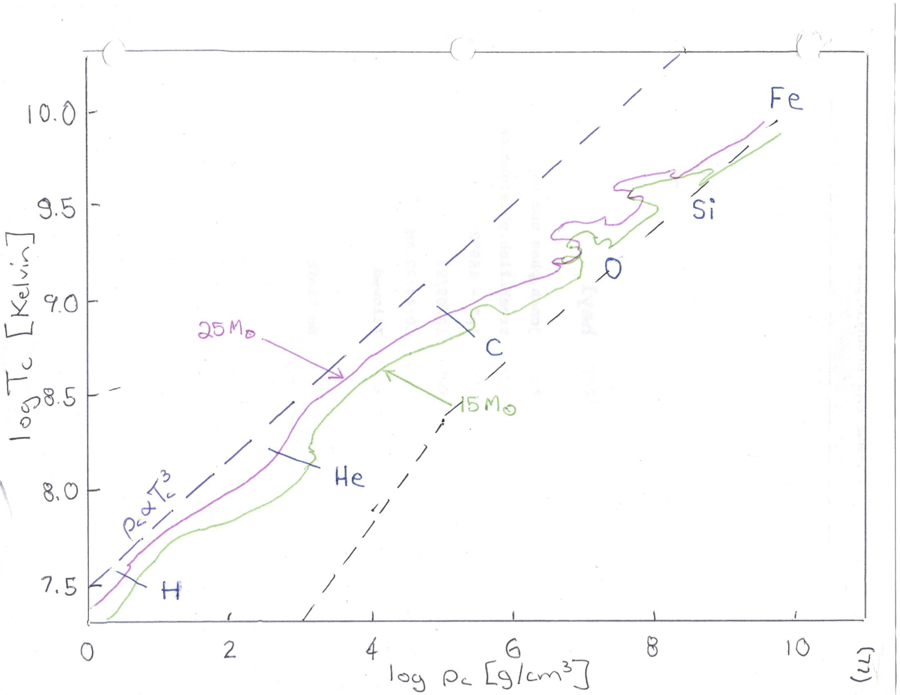
Let's build upon the solar models that you performed in Week 2. Run the a one-solar-mass model using 1M_pre_ms_to_wd. Idenify the various regions on the H-R diagram for the main sequence, giant branch, horizontal branch and asymptotic giant branch and plot the profiles of density, temperature, energy generation as a function of radius for each stage. Also plot temperature against density on a log-log plot to identify the convective and radiative regions.
Repeat the analysis for a 0.3 solar-mass star and a 3 solar-mass star.
Post-Main Sequence Evolution
Reading Assignment
Chapter 12 of Stellar-Astrophysics Notes
Low-Mass Stars
Core Contraction/Envelope Expansion
Oscillations
Reading Assignment
Chapter 13 of Stellar-Astrophysics Notes
Radial, Adiabatic Oscillations
Let's start with radial oscillations. We will use the enclosed mass as the coordinate and we can write
and write the equation of motion of a shell of fluid (hydrostatic equilibrium if no oscillation)
Substituting the perturbed expressions and keeping only the first-order terms gives
If we use the unperturbed equation and define
and
where we used the zeroth-order continuity equation
Now if we linearize this equation we get
and
We now have two equations but three unknowns and . The final ingredient is the equation of state which for an adiabatic gas gives
so now we can write the first equation just in terms of :
We can rewrite this and a Sturm-Liouville equation
This is an eigenvalue equation for the function . There are a countably infinite number of eigenvalues, all real. We will order this such that . The smallest eigenvalue will correspond to an eigenfunction without any nodes and similarly will correspond to an eigenfunction with nodes. Furthermore, these eigenfunctions will be orthogonal with the weighting over the interval .
Let's integrate all three terms times from to for the eigenfunction to get
and
If we take the adiabatic index to be constant and use the equation of hydrostatic equilibrium, we get
Because has no nodes, has the same sign as ; therefore means that for all of the modes are positive (all stable) and for at least and other might be too (at least one unstable mode).
Let's write everything in terms of dimensionless variables
to get
We see that is a constant for homologous stars. For polytropes one can also get the frequencies of the overtones
where is a dimensionless eigenvalue that depends only on and .
Can we estimate the frequencies in general for modes with many nodes? Let's use a variational principle and guess the eigenfunction to be
If we substitute this into the homologous frequency equation and integrate the denominator by parts twice we will get
Radial, Non-Adiabatic Oscillations
The key idea here is that for the modes to be sustained, they must not be strictly adiabatic! We can imagine the mode is like an engine and work must be done to drive the oscillation so heat must enter the gas at high temperature. For this to work the gas must be more opaque at the high temperature, high density part of the oscillation. We have
and
so
Therefore, the opacity will be smaller at the high density if , and this is typically the case.
However, an exception is a partially ionised layer. The compression ionises the layer but the temperature does not increase. Heat is absorbed during the compression and released during the expansion. This is called the mechanism.
H-ionization zone at 10,000-15,000 K: HI to HII and He I to He II.
He-ionization zone at 40,000 K: He II to He III
For these zone are too close to surface not much mass!
For these zone are deeper and the fundamental can be excited. There is in instability strip around effective temperatures between 5,500 and 7,500 K.
Non-Radial, Adiabatic Oscillations
Now things get more complicated, but we will make some simplifications to make our lives easier. First, the equations
Remember that the unperturbed solution is just a function of radius . We can follow the changes in the fluid in two ways, the Eulerian (I'm standing at a point) and Lagrangian (I'm moving with the fluid). We will use the prime to denote the Eulerian perturbation and to denote the Lagrangian perturbation. We can relate them by
where is the perturbation of the fluid from its equilibrium position. We can also think of changes in time as measured by someone in the fluid and someone standing still
We will connect the perturbation of the pressure to that of the density
We can now write perturbed Euler equation
and we can connect the density perturbation to the displacement field through the continuity equation
We would also need to calculate the perturbation to the gravitational potential through the Poisson equation, but we will make the Cowling approximation in which we take and we write
and get equations for the three components of the displacement
where
Notice that if the unperturbed star is adiabatic.
We can solve the two angular equations by using spherical harmonics
and
where the transverse component is related to by
so we can focus on and yielding the following two equations
and
where we have defined the Brunt-Vaisala frequency , the Lamb frequency and the transverse wavenumber as
and
The Brunt-Vaisala frequency is simply the oscillation frequency of a blob displaced vertically
and the Lamb frequency is the frequency of sound waves travelling transversely.
Unlike the equation for purely radial modes, this is not a Sturm-Liouville equation, so we have no guarantee that the value of is bounded from below. All that we do know is that is real and that the solutions will be orthogonal.
We can talk about modes with which will be constant on lines of constant latitude (). These are called zonal modes. We can also have modes with . These are constant on lines of longitude and are called sectoral modes. The other modes are called tesseral modes.
To make some further progress we will take a WKB approximation in which the radial variation is proportional to in the limit where . This yields a dispersion relation for the radial wavenumber
For a wave that is oscillatory in time we have . Furthermore for it to be oscillatory in the radial direction as well, we must have ; therefore, we can have waves for values of outside the range in between and . We have two types of waves those with greater than both and and those with less than both and . Usually we have . In this case we call the first modes or pressure modes and the second we call modes or gravity modes.
If we assume that we have
and
The size of the perturbations for the two types of modes are given by
We can approximate the number of radial nodes as
and the frequencies as
and
Check out the latest Doppler images of the Sun at http://jsoc.stanford.edu/data/hmi/images/latest/
Assignment
You will use the inlist called astero_adipls for this assignment. This model evolves a 1.2 solar mass star from the ZAMS until the hydrogen is nearly exhausted in the centre. I would like you to plot the sound speed (profile column csound) and Brunt frequency (brunt_N2) as a function of radius for the initial stage (ZAMS) , halfway through the evolution and at the final stage. Identify the convectively unstable regions on the plots. Plot the Lamb frequency for l=1,2,3. Identify the turning points of p-mode with ω=3000μHz for different values of angular momentum. What about 10,000μHz? Similarly what are the turning points of a 2000μHz g-mode?
Plot the structure of the first several modes (l=0, n=0 to 6) for the final model. The results are in the file ttt.adipls.prt.
High-Mass Stars
Reading Assignment
The evolution and explosion of massive stars, Sec I. to IV.
Complications
Semiconvection
Convective Overshoot
Diffusion
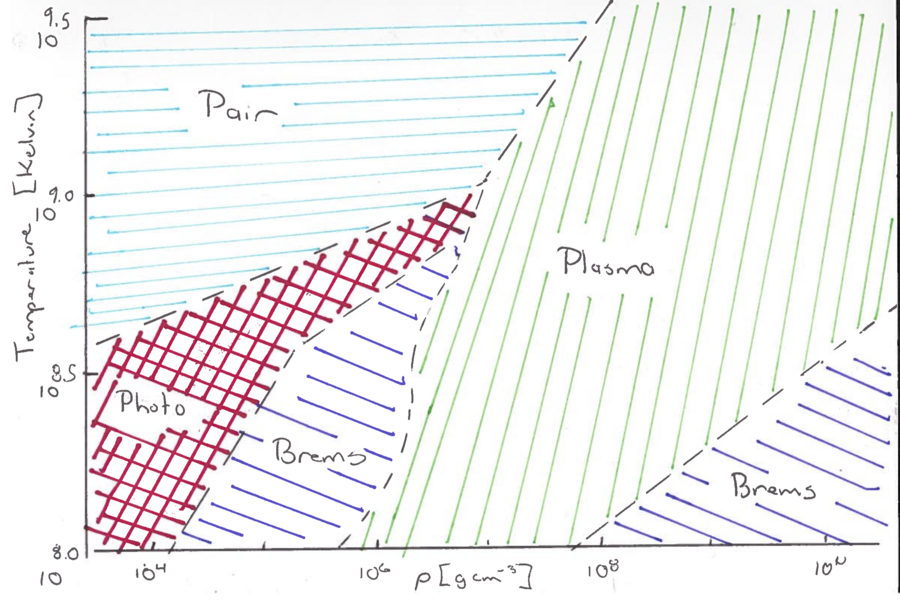
Neutrino Emission
Two basic processes:
- photo-neutrino: pair-annihilation, plasmon, bremsstrahlung
- Urca process: direct and modified
Assignment
You will create a 7 solar-mass star from the 7M_prems_to_AGB test suite
First, recall the various regions on the H-R diagram that you identified in the assignment for the solar mass star. Plot the solar mass star and the 7 solar mass star on the same H-R diagram. How does the behaviour of the two models differ?
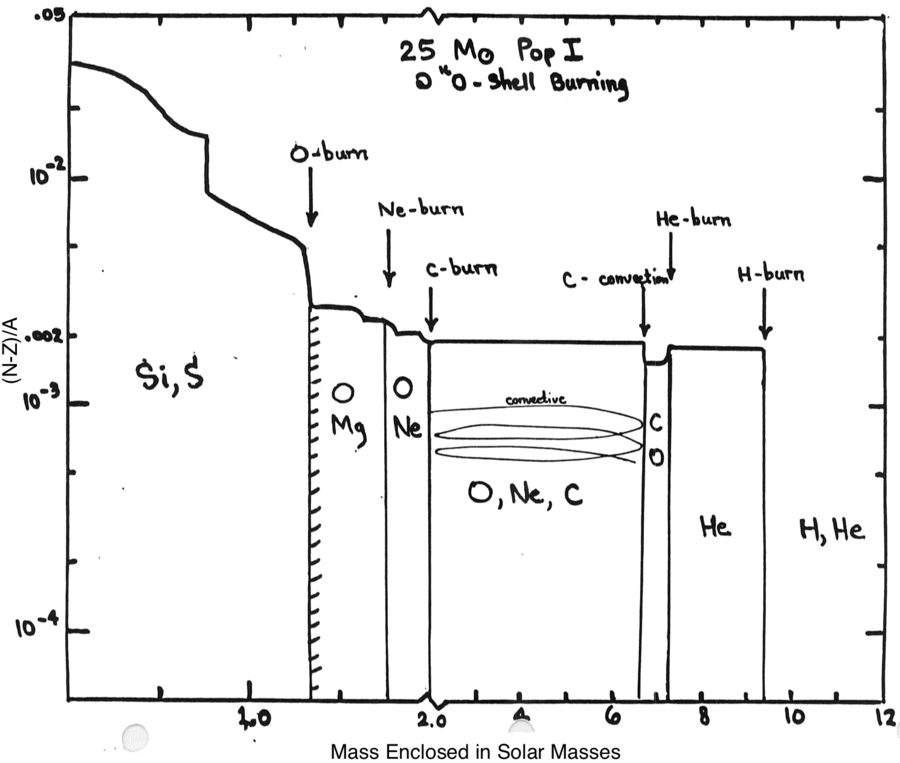
Plot the profiles of density, temperature, energy generation (dividing into the various reactions using the burn columns of the profile files) as a function of enclosed mass for the main sequence of the 7 solar-mass star and pick two later stages that you find interesting. Make a plot showing the composition of the different regions with the enclosed mass as the x-coordinate.
Plot temperature against density on a log-log plot to identify the convective and radiative regions. Plot neutrino luminosity as a function of time and compare with the one-solar-mass model (from the history file).
Supernovae
Reading Assignment
- Chapters 12 and 13 from Jim Lattimer's notes
- The evolution and explosion of massive stars, Sec V. to X.
- Type Ia Supernova Explosion Models
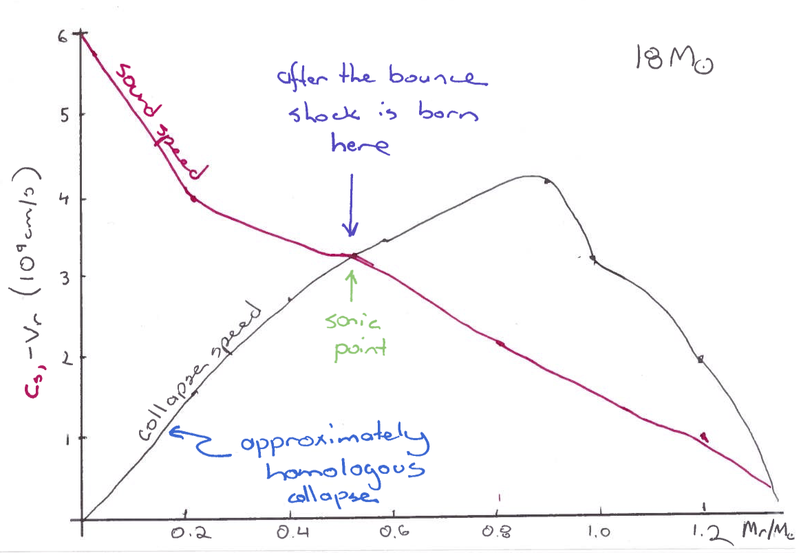
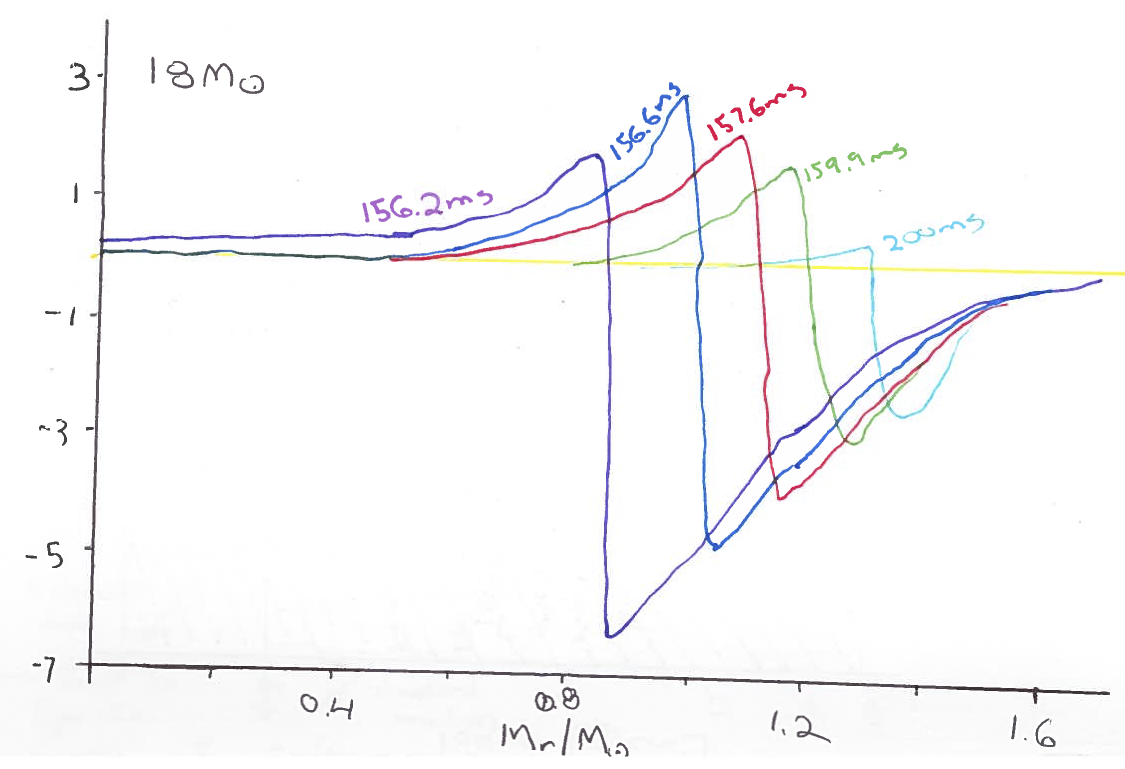
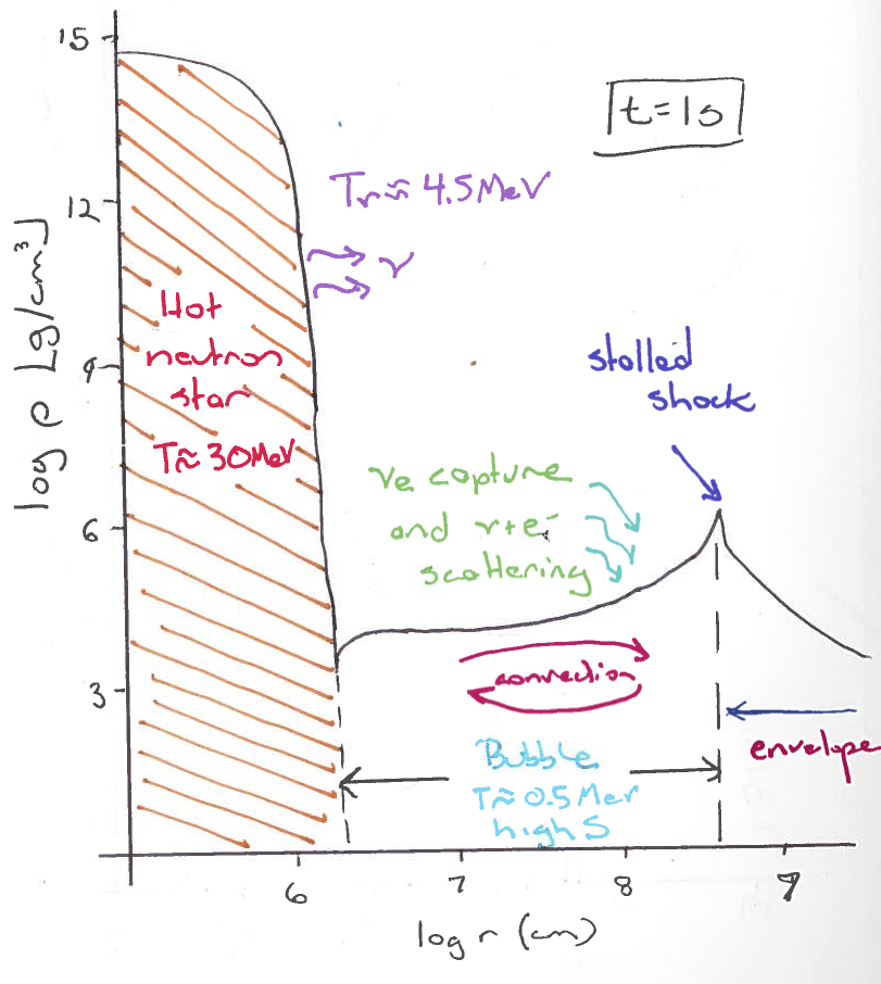
Core-Collapse
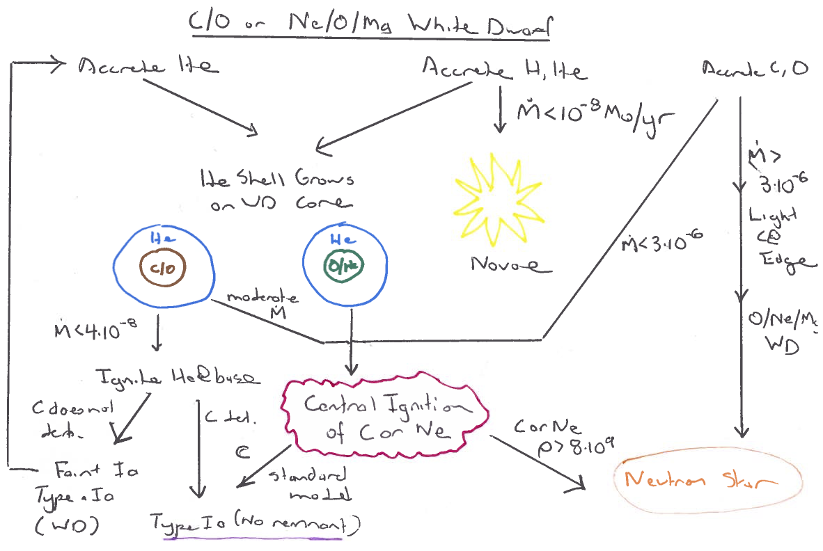
Thermonuclear
Assignment
For your assignment I would like you to focus on the following two inlists:
- wd_c_core_ignition (only about 3 minutes to run),
- split_burn_big_net_30M (only about 8 minutes to run).
For both runs I want you to add the dynamic timescale and the nuclear timescale to the history file. For the wd_c_core_ignition run only, I want you to add the various non-nuclear neutrino processes to the profile file.
Now how do you do this? In each of the directories you will have to edit files called history_columns.list and profile_columns.list. The wd_c_core_ignition by default only gives a few profiles. We want more so change profile_interval to 10 from 50 in the inlist file. You will have to make a few changes to split_burn_big_net_30M to get it to run to collapse. Hint: look at the stopping conditions.
For all of the plots I would like for you to use the enclosed mass as the abscissa.
For the the wd_c_core_ignition run,
- I would like for you to plot the neutrino losses through the star for the final profile for each of the processes.
- I would also like you to plot the various nuclear reaction rates for both the final profile and the second to last profile.
- Which nuclear reaction do you think is driving the instability? Are you surprised?
For the split_burn_big_net_30M I would like you to plot the various nuclear reaction rates, the composition and the specific entropy of the material as a function of the enclosed mass for the initial profile, one in the middle and the final profile.
- How much time has elapsed between the beginning of silicon burning and the collapse of the core? To get the core to collapse, you will probably have to change the inlist. Right now, it will stop after only a few models.
- Do you notice a mass at which the specific entropy abruptly rises near the centre? What is the significance of this mass?
- Can you infer from the specific entropy curve what is happening in the different regions? Hint: compare it with the nuclear burning profiles.
Nucleosynthesis
Reading Assignment
Synthesis of the elements in stars: forty years of progress, George Wallerstein, Icko Iben, , Jr., Peter Parker, Ann Merchant Boesgaard, Gerald M. Hale, Arthur E. Champagne, Charles A. Barnes, Franz Käppeler, Verne V. Smith, Robert D. Hoffman, Frank X. Timmes, Chris Sneden, Richard N. Boyd, Bradley S. Meyer, and David L. Lambert Rev. Mod. Phys. 69, 995 – Published 1 October 1997
Introduction
http://adsabs.harvard.edu/abs/1957RvMP...29..547B
http://adsabs.harvard.edu/abs/1965ApJS...11..121S
http://adsabs.harvard.edu/abs/1999PrPNP..43..419K
http://adsabs.harvard.edu/abs/2007PhR...450...97A
α-process
The alpha process is one of two classes of nuclear fusion reactions by which stars convert helium into heavier elements, the other being the triple-alpha process. While the triple-alpha process only requires helium, once some carbon is present, these other reactions that consume helium are possible:
E is the energy produced by the reaction, released primarily as gamma rays (Template:Mvar).
This sequence ends at because it is the most stable (i.e., it has the highest nuclear binding energy per nucleon) in the chain. has the most binding energy per nucleon and has the least mass per nucleon. Therefore, production of heavier nuclei requires energy instead of releasing it.
All these reactions have a very low rate at the temperatures and densities in stars and therefore do not contribute significantly to a star's energy production; with elements heavier than neon (atomic number > 10), they occur even less easily due to the increasing Coulomb barrier.
Alpha process elements (or alpha elements) are so-called since their most abundant isotopes are integer multiples of four, the mass of the helium nucleus (the alpha particle). They are synthesized by alpha capture prior to silicon burning a precursor to Type II supernovae. Silicon and calcium are purely alpha process elements. Magnesium can be burned by proton capture reactions. As for oxygen, some authorsTemplate:Which consider it an alpha element, while others do not. Oxygen is surely an alpha element in low-metallicity population II stars. It is produced in Type II supernovae and its enhancement is well correlated with an enhancement of other alpha process elements. Sometimes carbon and nitrogen are considered alpha process elements, since they are synthesized in nuclear alpha-capture reactions.
The abundance of alpha elements in stars is usually expressed in a logarithmic manner:
- ,
Here and are the number of alpha elements and iron nuclei per unit volume. Theoretical galactic evolution models predict that early in the universe there were more alpha elements relative to iron. Type II supernovae mainly synthesize oxygen and the alpha-elements (Ne, Mg, Si, S, Ar, Ca and Ti) while Type Ia supernovae mainly produce elements of the iron peak: TI, V, Cr, Mn, Fe, Co and Ni, but also alpha-elements
s-process
Carbon-13 pocket
r-process
p-process
rp-process
Cosmic-Ray Spallation
Assignment
- For elements with atomic numbers less than that of calcium, the most abundant isotope of each element with an even number of protons has Z=N, e.g. 4He, 12C, 16O, 40Ca, ... and those with odd proton numbers, N, Na, Al ... have Z nearly equal to N. When one goes to heavier nuclei however there is a surplus of neutrons in the most abundant isotopes; iron-56 has 26 protons and 30 neutrons. Explain both these trends why light nuclei have Z about equal to N while heavy nuclei have Z less than N.
- Why is combination of a single neutron and a single proton stable but two protons is not?
- Calculate the energy released in erg/g when a composition of pure helium burns to pure carbon-12 and to 50/50 carbon-12 and oxygen 16. What is the energy released when each of these mixtures is burned to Nickel-56? In both cases how much nickel has to be made to produce 1051 erg?
- The neutron capture cross sections at 30 keV for the stable isotopes of barium are 130Ba, 715 mb 132Ba, 447mb, 134Ba, 221 mb 135Ba, 457 mb, 136Ba, 69 mb, 137Ba, 57 mb, and 138Ba, 3.9 mb. The s-only isotopes of barium are 134 and 136 and the nuclear charge is 56. a) Why is the cross section of 135Ba greater than that of 134Ba or 136Ba? Why is the cross section of 138Ba so small? What do you expect for the solar ratio of the abundance of 134Ba to that of 136Ba? Your discussion should at least mention why reactions with large releases of energy have large cross-sections.
