2.3 Some Common Continuous Distributions
Let us consider some common continuous random variables that often arise in practice. We should stress that this is indeed a very small sample of common continuous distributions.
The Beta Distribution
Suppose the proportion p of restaurants that make a profit in their first year of operation is given by a certain beta random variable X, with probability density function:
What is the probability that more than half of the restaurants will make a profit during their first year of operation? To answer this question, we calculate the probability as an area under the PDF curve as follows:
Therefore, Pr(0.5 ≤ P ≤ 1) = 0.3125.
The example above is a particular case of a beta random variable. In general, a beta random variable has the generic PDF:
where the constants a and b are greater than zero, and the constant k is chosen so that the density f integrates to 1.
We see that our previous example was a beta random variable given by the above density with a = 2 and b = 3. Let us find the associated cumulative distribution function F(p) for this random variable. We compute:
valid for 0 ≤ p ≤ 1.
The Exponential Distribution
The lifespan of a lightbulb can be modeled by a continuous random variable since lifespan - i.e. time - is a continuous quantity. A reasonable distribution for this random variable is what is known as an exponential distribution.
A random variable Y has an exponential distribution with parameter β > 0 if its PDF is given by
Suppose that the lifespan (in months) of lightbulbs manufactured at a certain facility can be modeled by an exponential random variable Y with parameter β = 4. What is the probability that a particular lightbulb lasts at least a year? Again, we can calculate this probability by evaluating an integral. Since there are 12 months in one year, we calculate
Thus we can see that it is highly likely we would need to replace a lightbulb produced from this facility within one year of manufacture.
The Continuous Uniform Distribution
Our third example of a common continuous random variable is one that we have already encountered. Consider the experiment of randomly choosing a real number from the interval [a,b]. Letting X denote this random outcome, we say that X has a continuous uniform distribution on [a,b] if the probability that we choose a value in some subinterval of [a,b] is given by the relative size of that subinterval in [a,b]. More explicitly, we have the following:
A random variable X has an continuous uniform distribution on [a,b] if its PDF is constant on [a,b]; i.e. its PDF is given by
The continuous uniform distribution has a particularly simple representation, just as its discrete counterpart does. Nevertheless, this random variable has great practical and theoretical utility. We will explore this distribution in more detail in the following example and in the exercises.
A Geometric Problem
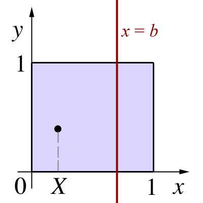
Consider the square in the xy-plane bounded by the lines x = 0, x = 1, y = 0 and y = 1. Now consider a vertical line with equation x = b, where 0 ≤ b ≤ 1 is fixed. Note that this line will intersect the unit square just defined.
Suppose we select a point inside this square, uniformly at random. If we let X be the x-coordinate of this random point, what is the probability that X is in the interval [0 , b]?
An illustration of our problem is given in the figure below. Graphically, we are trying to find the probability that a randomly selected point inside the square lies to the left of the red line.
The region to the left of the red line is a rectangle with area equal to b. The probability that our random point lies inside this rectangle is proportional to the area of that rectangle, since the larger the area of the rectangle, the larger the probability is that the point is inside of it.
- If the probability that the point is between 0 and b were equal to 0.5, then the red line would have to divide the square into two equal halves: so b = 0.5.
- If the probability that the point is between 0 and b were equal to 0.25, then the red line would have to divide the square at 1/4: so b = 0.25.
- If the probability that the point is between 0 and b were equal to 1, then the red line would have to lie on the rightmost edge of the square itself: so b = 1
In general, we see that we should have Pr(0 ≤ X ≤ b) = b.
Notice that this result matches with the definition of our random variable X. Since we want to select a random point uniformly at random from the unit square, the random variable X giving the x-coordinate of this random point should be a continuous uniform random variable on the interval [0,1]. Thus, the PDF of X is simply , where .
Therefore, , which agrees with the answer we derived using purely geometric considerations.
