2.1 - The Cumulative Distribution Function of a Continuous Random Variable

In the previous chapter, we defined random variables in general, but focused only on discrete random variables. In this chapter, we properly treat continuous random variables.

If for example X is the height of a randomly selected person in British Columbia, or X is tomorrow's low temperature at Vancouver International Airport, then X is a continuously varying quantity.

We previously defined a continuous random variable to be one where the values the random variable can assume are given by a continuum of values. For example, we can define a continuous random variable that can take on any value in the interval [1,2].

To make this definition more precise, we recall the definition from Section 1.4 of a cumulative distribution function (CDF) that was given for any random variable.

The Cumulative Distribution Function
The cumulative distribution function for any random variable X, denoted by F(x), is the probability that X assumes a value less than or equal to x: $F(x)={\text{Pr}}(X\leq x)$ The cumulative distribution function has the following properties: 0 ≤ F(x) ≤ 1 for all values of x $\lim _{x\rightarrow -\infty }F(x)=0$ $\lim _{x\rightarrow +\infty }F(x)=1$ F(x) is a nondecreasing function of x

This definition is independent of the type of random variable to which we are referring. From this, we can define a continuous random variable to be any random variable X whose CDF is a continuous function. Notice that this is in contrast to the case of discrete random variables where the corresponding CDF is always a discontinuous step-function.

Continuous Random Variable
A continuous random variable is one that has a continuous cumulative distribution function.

Comparison to the Discrete Case

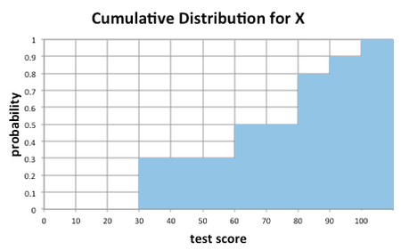
Recall the cumulative distribution function we had for the test scores example in the previous chapter. The graph of the cumulative distribution function is given below.

Observe that the graph of this function "increases in steps" at 30, 60, 80, 90, and 100. CDFs for discrete random variables are always step functions. A discrete random variable cannot assume a continuum of values; thus, its CDF can only increase at a finite or countably infinite set of points.

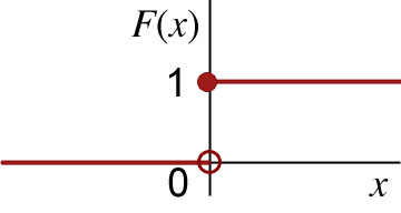
For another example, consider the function whose graph is given below.

This function cannot represent a CDF for a continuous random variable because the function F is not continuous for all values of x. However, F could represent a cumulative distribution function for a discrete random variable since it increases from 0 to 1 in a finite number of steps.

Example: Maximum Outdoor Air Temperature

The maximum outdoor air temperature in downtown Vancouver on any given day in January can be expressed as a continuous random variable X. A reasonable CDF for this random variable is given by the function

$F(x)={\frac {1}{1+e^{-kx}}},\ {\text{ for some }}k>0$

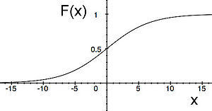
For a particular k, we have graphed this cumulative distribution function in the plot below.

In the above plot, note that the horizontal x-axis gives possible values of the maximum outdoor air temperature in downtown Vancouver on any day in January, and that the vertical probability-axis gives values between 0 and 1. The value of the cumulative distribution function F(x) gives the probability that the maximum outdoor air temperature is no greater than x.

We can easily see that this function satisfies the basic properties of a CDF. Clearly, F(x) ≥ 0 for all possible temperatures x. Also, F(x) ≤ 1 for all x since the denominator in the definition of F(x) is always larger than the numerator. Since k > 0, we calculate

$\lim _{x\rightarrow -\infty }F(x)=\lim _{x\rightarrow -\infty }{\frac {1}{1+e^{-kx}}}=0.$

Likewise,

$\lim _{x\rightarrow +\infty }F(x)=\lim _{x\rightarrow +\infty }{\frac {1}{1+e^{-kx}}}=1.$

To check that F is nondecreasing, we note that since F is everywhere differentiable, it suffices to show that the derivative of F is nonnegative. A quick calculation yields

${\frac {d}{dx}}F(x)={\frac {ke^{-kx}}{(1+e^{-kx})^{2}}}$

which is certainly never negative. Thus we see explicitly that this function F(x) satisfies all the basic properties that a CDF should.