1.4 The Cumulative Distribution Function

Generally speaking, for any random variable X, we define the cumulative distribution function (CDF) of X as follows:

Cumulative Distribution Function
The cumulative distribution function (CDF) of a random variable X is denoted by F(x), and is defined to be the function $F(x)={\textrm {Pr}}(X\leq x).$

In other words, the cumulative distribution function for a random variable at x gives the probability that the random variable X is less than or equal to that number x.

Given a discrete random variable and its associated probability mass function, the definition of the cumulative distribution function can be rewritten using our identity for the probability of disjoint events (see Section 1.02).

Cumulative Distribution Function of a Discrete Random Variable
If X is a discrete random variable, the cumulative distribution function (CDF) of X can be written as $F(x)=\sum _{k=1}^{n}{\textrm {Pr}}(X=x_{k})$ where x_n is the largest possible value of X that is less than or equal to x.

Note that in this formula for CDFs of discrete random variables, we always have $n\leq N\!$ , where N is the number of possible outcomes of X.

Notice also that the CDF of a discrete random variable will remain constant on any interval of the form $[x_{n},x_{n+1})\!$ . That is, $F(x)=F(x_{n})=\sum _{k=1}^{n}{\textrm {Pr}}(X=x_{k}){\text{ for any }}x\in [x_{n},x_{n+1})\!$ .

The following properties are immediate consequences of our definition of a random variable and the probability it associates to an event.

Properties of the CDF
$0\leq F(x)\leq 1{\text{ for all }}x$ $\lim _{x\rightarrow -\infty }F(x)=0$ $\lim _{x\rightarrow +\infty }F(x)=1$ F(x) is a nondecreasing function of x

Recall that a function f(x) is said to be nondecreasing if f(x₁) ≤ f(x₂) whenever x₁ < x₂.

Example: Rolling a Single Die

If X is the random variable we associated previously with rolling a fair six-sided die, then we can easily write down the CDF of X.

We already computed that the PMF of X is given by Pr(X = k) = 1/6 for k = 1,2,...,6. The CDF can be computed by summing these probabilities sequentially; we summarize as follows:

Pr(X ≤ 1) = 1/6
Pr(X ≤ 2) = 2/6
Pr(X ≤ 3) = 3/6
Pr(X ≤ 4) = 4/6
Pr(X ≤ 5) = 5/6
Pr(X ≤ 6) = 6/6 = 1

Notice that Pr(X ≤ x) = 0 for any x < 1 since X cannot take values less than 1. Also, notice that Pr(X ≤ x) = 1 for any x > 6. Finally, note that the probabilities Pr(X ≤ x) are constant on any interval of the form [k,k + 1) as required.

Example: Rolling Two Dice

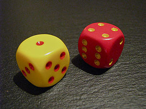
Suppose that we have two fair six-sided dice, one yellow and one red as in the image below.

We roll both dice at the same time and add the two numbers that are shown on the upward faces.

Let Y be the discrete random variable associated to this sum.

How many possible outcomes are there? That is, how many different values can Y assume?
How is Y distributed? That is, what is the PMF of Y?
What is the probability that Y is less than or equal to 6?
What is the CDF of Y?

Solution

Part 1)

There are 6 possible values we can observe of each die. The two dice are rolled independently (i.e. the value on one of the dice does not affect the value on the other die), so we see that there are 6 ✕ 6 = 36 different outcomes for a single roll of the two dice. Notice that all 36 outcomes are distinguishable since the two dice are different colors. So we can distinguish between a roll that produces a 4 on the yellow die and a 5 on the red die with a roll that produces a 5 on the yellow die and a 4 on the red die.

However, we are interested in determining the number of possible outcomes for the sum of the values on the two dice, i.e. the number of different values for the random variable Y. The smallest this sum can be is 1 + 1 = 2, and the largest is 6 + 6 = 12. Clearly, Y can also assume any value in between these two extremes; thus we conclude that the possible values for Y are 2,3,...,12.

Part 2)

To determine the probability distribution for Y, first consider the probability that the sum of the dice equals 2. There is only one way that this can happen: both dice must roll to 1. There are 36 distinguishable rolls of the dice, so the probability that the sum is equal to 2 is 1/36.

The other possible values of the random variable Y and their corresponding probabilities can be calculated in a similar fashion. Some of these are listed in the table below.

Outcome (Yellow, Red)	Sum = Yellow + Red	Probability
(1,1)	2	1/36
(1,2), (2,1)	3	2/36
(1,3), (2,2), (3,1)	4	3/36
(1,4), (2,3), (3,2), (4,1)	5	4/36
(1,5), (2,4), (3,3), (4,2), (5,1)	6	5/36
. . .	. . .	. . .
(6,6)	12	1/36

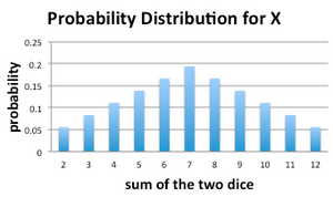
The probability mass function of Y is displayed in the following graph.

Alternatively, if we let p_k = Pr(Y = k), the probability that the random sum Y is equal to k, then the PMF can be given by a single formula:

$p_{k}={\frac {6-|k-7|}{36}}{\text{ if }}k=2,3,\ldots ,12$

Part 3)

The probability that the sum is less than or equal to 6 can be written as Pr( Y ≤ 6), which is equal to F(6), the value of the cumulative distribution function F(y) of Y at y = 6. Using our identity for probabilities of disjoint events, we calculate

$\mathrm {Pr} (Y\leq 6)=F(6)=\sum _{k=1}^{6}p_{k}=0+{\frac {1}{36}}+{\frac {2}{36}}+{\frac {3}{36}}+{\frac {4}{36}}+{\frac {5}{36}}={\frac {15}{36}}={\frac {5}{12}}$

Part 4)

To find the CDF of Y in general, we need to give a table, graph or formula for F(k) = Pr(Y ≤ k) for any given k. Using our table for the PMF of Y, we can easily construct the corresponding CDF table:

Y = k	F(k) = Pr(Y ≤ k)
2	1/36
3	3/36
4	6/36
5	10/36
6	15/36
. . .	. . .
12	36/36 = 1

This table defines a step-function starting at 0 for y < 2 and increasing in steps to 1 for y ≥ 12. Notice that the CDF is constant over any half-closed integer interval from 2 to 12. For example, F(y) = 3/36 for all y in the interval [3,4).

Example: Test Scores

Consider the example of selecting a test score from a given collection that we explored in the previous section: in a class of 10 people, grades on a test were 30, 30, 30, 60, 60, 80, 80, 80, 90, 100. Let X be the score of a randomly drawn test from this collection.

Calculate the probability that a test drawn at random has a score less than or equal to 80.
Calculate the probability that a test drawn at random has a score less than or equal to x_n, where x_n = 0, 10, 20, 30, ... , 100.

Solution

Part 1)

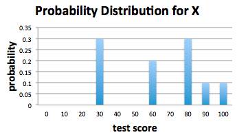
Recall the probability mass function, calculated earlier:

Let p_k be the probability that the score of a randomly drawn test is x_k = 10k. So, for example:

p₀ is the probability that a randomly drawn test score is 0
p₁ is the probability that a randomly drawn test score is 10
p₂ is the probability that a randomly drawn test score is 20
p₃ is the probability that a randomly drawn test score is 30

and so on. Values for each of these probabilities are given in the above bar graph. Notice that many of these probabilities are zero.

The probability that a test drawn at random has a score of no greater than 80 is exactly the value of the CDF of X at x = 80; i.e.,

${\begin{aligned}\mathrm {Pr} (X\leq 80)&=F(80)\\&=\sum _{k=0}^{8}p_{k}\\&=p_{0}+p_{1}+p_{2}+{\color {Blue}{p_{3}}}+p_{4}+p_{5}+{\color {Blue}{p_{6}}}+p_{7}+{\color {Blue}{p_{8}}}\\&=0+0+0+\mathbf {\color {Blue}{\frac {3}{10}}} +0+0+{\color {Blue}{\frac {2}{10}}}+0+{\color {Blue}{\frac {3}{10}}}\\&={\frac {8}{10}}\\&={\frac {4}{5}}\end{aligned}}$

The color blue was used in the above calculation to highlight nonzero probabilities.

Because of the sample space of our experiment, if the randomly selected grade is to be less than or equal to 80, then this grade can only be 30, 60, or 80. Intuitively, the probability that a randomly selected test has a grade of 30, 60, or 80 is the sum of the probabilities that the score is one of these possibilities, which we note is in agreement with our identity concerning probabilities of disjoint events from Section 1.02.

Part 2)

Now we want to calculate the probability that a test drawn at random has a score less than or equal to x_k = 10k for k = 0,1,...,10. Again, we identify this as simply finding the value of the CDF of X at each of these x_k values.

$\mathrm {Pr} (X\leq 0)=F(0)=\sum _{k=0}^{0}p_{k}=p_{0}=0$

Similarly, $F(0)=F(10)=F(20)=0$ . F(30) is non-zero:

$\mathrm {Pr} (X\leq 30)=F(30)=\sum _{k=0}^{3}p_{k}=0+0+0+{\frac {3}{10}}$

Notice that F(40) is equal to F(30), since p₄ = 0.

Other values of F are calculated in the same way using the definition of the cumulative distribution function. The following table contains the values of the CDF of X for x_k = 0, 10, 20, 30, ... 100.

k	x_k	F(x_k)
0	0	0
1	10	0
2	20	0
3	30	0.3
4	40	0.3
5	50	0.3
6	60	0.5
7	70	0.5
8	80	0.8
9	90	0.9
10	100	1.0

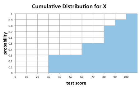
Collectively, our calculations give the CDF of the random variable X. This cumulative distribution function is graphed in the figure below.