Course:CPSC522/IsAttentionExplanation

Title: Is Attention Explanation?

This page is about determining if attention weights in a Natural Language Processing (NLP) model can provide meaningful explanations for predictions with the help of certain tests. The two papers that will be discussed in this page are:

• Sarthak Jain and Byron C. Wallace. 2019. Attention is not Explanation. In Proceedings of the 2019 Conference of the North American Chapter of the Association for Computational Linguistics: Human Language Technologies, Volume 1 (Long and Short Papers), pages 3543–3556, Minneapolis, Minnesota. Association for Computational Linguistics.
• Sarah Wiegreffe and Yuval Pinter. 2019. Attention is not not Explanation. In Proceedings of the 2019 Conference on Empirical Methods in Natural Language Processing and the 9th International Joint Conference on Natural Language Processing (EMNLP-IJCNLP), pages 11–20, Hong Kong, China. Association for Computational Linguistics.

Principal Author: Harshinee Sriram

Abstract

This page explores the relevance of attention weights in an NLP model when it comes to explaining the predictions made by the model. The first research paper introduces some tests to determine the significance of attention weights and argues that standard attention modules do not provide meaningful explanations for model predictions and, hence, it is erroneous to consider them as a method to provide insights on the model's internal decision process that led to a certain output. The second research paper challenges several assumptions that the first paper was based on, improves the proposed tests, and introduces a few new tests to ultimately argue that attention is, indeed, a valuable tool for understanding the behavior of neural network models.

Builds on

• Deep Learning (DL) is part of a broader family of machine learning methods based on artificial neural networks with representation learning. Learning can be supervised, semi-supervised or unsupervised.
• Natural language processing (NLP) is an interdisciplinary subfield of linguistics, computer science, and artificial intelligence concerned with the interactions between computers and human language, in particular how to program computers to process and analyze large amounts of natural language data.

Related Pages

• Artificial Neural Networks (or simply Neural Networks/NN) are computing systems inspired by the biological neural networks that constitute animal brains. An ANN is based on a collection of connected units or nodes called artificial neurons, which loosely model the neurons in a biological brain.
• A Long Short-Term Memory (LSTM) is a type of recurrent neural network that is capable of remembering past information and processing sequences of data. It uses gates to control the flow of information, allowing it to maintain a balance between retaining important information and discarding irrelevant data, making it well-suited for tasks that involve sequential data such as language modeling and speech recognition.
• Explainable AI (XAI) is artificial intelligence (AI) in which humans can understand the decisions or predictions made by the AI.
• Attention is a technique that is meant to mimic cognitive attention. The effect enhances some parts of the input data while diminishing other parts — the motivation being that the network should devote more focus to the small, but important, parts of the data.

Content

Introduction

Using attention weight distributions to generate heatmaps over the input - used to explain what parts of the input the model considered most important for the resulting output. Source: https://dennybritz.com/posts/wildml/attention-and-memory-in-deep-learning-and-nlp/

Attention in NLP refers to a mechanism in deep learning models that allows the model to focus on specific parts of the input data. This helps the model predict by considering only the most relevant information. Attention is commonly used in NLP tasks such as machine translation, text classification, and sentiment analysis. Attention mechanisms are designed to be flexible, allowing the model to dynamically adjust the importance of different parts of the input data. This has made attention a popular tool in NLP research and has led to significant advances in the field.

Attention weights are often perceived to be a gateway to understanding the "internal decision process" of models. This is because, for a given model prediction, one can inspect the inputs to which the model assigned most importance to in order to understand why the resulting prediction was made. As a result, there are several claims about attention providing deep learning model interpretability and they all share the underlying assumption that the input features with the highest attention weights are the most influential features for the generated output. The first paper (referred to as Jain & Wallace, 2019 from hereon) argues that the notion of attention being a faithful explanation method relies on the following two properties:

• Attention weights should correlate with other feature importance measures, and
• Alternate (or counterfactual) attention weights should correspond to alternate predictions. In the event that they lead to the same output, these alternate attention weights can be regarded as alternate explanations for that output.

The authors develop tests to asses these properties and find that none of these properties hold for a Bidirectional LSTM (BiLSTM) with a standard attention mechanism (architectural assumptions discussed in the next section) for the NLP tasks of text classification, question answering (QA), and Natural Language Inference (NLI). This leads them to question the underlying assumption that correlates input feature importance to attention weights and, hence, the authors caution against using attention weights as a faithful explanation method.

The second paper (referred to as Wiegreffe & Pinter, 2019 from hereon) argues that the claims made by Jain & Wallace (2019) depend on a specific definition for an explanation and that their tests fail to holistically analyze the impact of attention weights in a model. Hence, Wiegreffe & Pinter (2019) propose alternative tests to determine if attention weights can be used as an explanation method, and find that attention weights can provide a valuable way to decipher feature importance.

Preliminaries and assumptions

The two papers assume model inputs $x\,\epsilon \,R^{T\times |V|}$ to be composed of one-hot encoded words for each word in an input sequence of length $T$. These inputs are passed through an embedding matrix $E$ that provides dense token representations (each of which is $d$ dimensional) i.e. $x_{e}\,\epsilon \,R^{T\times d}$. Next comes the encoder ($Enc$) that takes the embedded tokens in order as input and produces $T$ $m$-dimensional hidden states i.e. $h=Enc(x_{e})\,\epsilon \,R^{T\times m}$. These papers predominantly consider a BiLSTM model as an encoder and also analyze unordered 'average' embedding variations in which $h_{t}$ is the embedding of token $t$ after it is passed through a linear projection layer and ReLU activation.

A similarity function $\phi$ maps $h$ and a query $Q\,\epsilon \,R^{m}$ (emerging from a natural language task such as a hypothesis in Natural Language Inference or NLI) to scalar scores. Then, attention is induced over these scores: ${\hat {\alpha }}\,=\,softmax(\phi (h,Q))\,\epsilon \,R^{T}$. Both works consider additive attention:

• Additive attention: $\phi (h,Q)\,=\,v^{T}tanh(W_{1}h\,+\,W_{2}Q)$

Where, $v,\,W_{1},\,W_{2}$ are model parameters. In addition, Jain & Wallace (2019) consider scaled dot-product attention (these results are comparable to those from additive attention, hence Wiegreffe & Pinter (2019) do not delve into this for their work):

• Scaled dot-product attention: $\phi (h,Q)\,=\,{\frac {hQ}{\sqrt {m}}}$

These scores with attention weights are then sent to a decoder ($Dec$) with parameters $\theta$, which yields a prediction ${\hat {y}}\,=\,\sigma (\theta \,\cdot \,h_{\alpha })\,\epsilon \,R^{|\gamma |}$. Here, $h_{\alpha }\,=\,\sum _{t=1}^{T}{\hat {\alpha }}\cdot h_{t}$; $\sigma$ is an output activation function, and $|\gamma |$ denotes the label set size.

Paper 1: Attention is not explanation.

Research questions

Jain & Wallace (2019) are specifically interested in whether attention weights indicate why a model made the prediction that it did by addressing the following two questions:

1. Do learned attention weights agree with other methods for understanding feature importance? (RQ1)
2. If different features were attended to (i.e., features with low corresponding attention weights), would the prediction have been different? (RQ2)

Datasets and Tasks

To answer their research questions, the authors use datasets corresponding to three NLP tasks: binary text classification, question answering, and natural language inference. These datasets have been briefly described below:

1. Binary text classification
   1. The Stanford Sentiment Treebank [SST] dataset consists of over 10,000 sentence-level annotations of sentiment polarity, ranging from very negative (score of 1 out of 5) to very positive (score of 5 out of 5), for movie reviews.
   2. The IMDB large movie reviews [IMDB] dataset is a popular benchmark dataset in sentiment analysis. It contains over 50,000 reviews of movies labeled as positive or negative.
   3. The Twitter Adverse Drug Reaction [ADR Tweets] dataset is a collection of tweets annotated for adverse drug reactions.
   4. The 20 newsgroups [20News] dataset is a collection of newsgroup posts that are divided into 20 different categories, including topics such as politics, religion, and sports.
   5. The AG News Corpus [Business vs World] dataset is a collection of 496,835 news articles from 2000+ sources labeled as either "business" or "world" news.
   6. The MIMIC ICD9 [Diabetes] dataset is a collection of electronic health records (EHRs) annotated with International Classification of Diseases, Ninth Revision (ICD9) codes for diabetes.
   7. The MIMIC ICD9 (Chronic vs Acute Anemia) [Anemia] dataset is a collection of electronic health records (EHRs) annotated with International Classification of Diseases, Ninth Revision (ICD9) codes for chronic and acute anemia.
2. Question Answering (QA)
   1. The CNN News articles [CNN] dataset is a collection of news articles published by the cable news network CNN.
   2. The bAbI [bAbI] dataset consists of 20 synthetic tasks that require the model to answer questions based on a given context using a single supporting fact for a question and two/three supporting statements connected to form a coherent line of reasoning.
3. Natural Language Inference (NLI)
   1. The SNLI (Stanford Natural Language Inference) [SNLI] dataset is a collection of sentence pairs with labeled relationships indicating whether the second sentence entails, contradicts, or is neutral with respect to the first sentence.

Answering RQ1: Do learned attention weights agree with other methods for understanding feature importance?

Algorithm 1: Feature Importance Computations. Source: https://arxiv.org/abs/1902.10186

To quantify the notion of if two weight distributions "agree" with each other, the authors measure the Kendall rank correlation between attention and two alternate feature importance determination methods (referred to as saliency methods from now on). Kendall rank correlation is a non-parametric correlation coefficient that assesses the similarity of the orderings of the two variables without assuming any specific distribution or functional form. It is based on counting the number of concordant and discordant pairs of observations between the two variables, and it ranges between -1 and 1, where -1 indicates a perfect negative correlation, 0 indicates no correlation, and 1 indicates a perfect positive correlation.

The two saliency methods selected are: gradient-based ($\tau _{g}$) and leave one out or LOO ($\tau _{loo}$), the latter of which presents differences in model output induced by leaving features out. The authors select these saliency methods because previous work shows that they provide measures of individual feature importance with known semantics.

Algorithm 1 shows this process. The algorithm denotes the input generated after removing the word at position $t$ in $x$ by $x_{t}$. Note that the computation graph is disconnected at the attention module so that the gradient does not flow through this layer. Hence, the gradients depict how predictions change as a function of the inputs while keeping the attention distribution fixed. Table 1 presents the summary statistics of Kendall $\tau$ correlations for each dataset whereas Figure 1 shows the full distributions in the form of $\tau _{g}$ histogram plots for every data point in the respective corpora. To view the the complete results, visit: https://successar.github.io/AttentionExplanation/docs/.

Figure 1: Histogram of Kendall τ between attention and gradients. Encoder variants are denoted parenthetically; colors indicate predicted classes. Source: https://arxiv.org/abs/1902.10186

Table 1: Mean and std. dev. of correlations between gradient/leave-one-out importance measures and attention weights. Sig. Frac. columns report the fraction of instances for which this correlation is statistically significant; note that this largely depends on input length, as correlation does tend to exist, just weakly. Encoders are denoted parenthetically. These are representative results. Source: https://arxiv.org/abs/1902.10186

In Figure 1, orange refers to instances predicted as positive and purple refers to those predicted as negative. For the SNLI dataset, the colours purple, orange, and green refer to contradiction, entailment, and neutral respectively. The authors observe that, in general, the obtained correlations are modest for the BiLSTM encoder. The observed densities are centered around or below 0.5 in most cases. Additionally, from Table 1, they find that as correlation is sufficiently weak, a statistically significant correlation cannot be consistently established across all datasets and tasks.

On the other hand, gradients in average embedding based models show very high degree of correspondence with attention weights with the correlation between LOO scores and attention weights being ~0.375 points higher for this encoder when compared to the BiLSTM encoder. The authors regard this observation to the possibility that both attention weights and average embeddings are simple encoders, whereas BiLSTM is a more complex encoder as it induces gradient-importance based on hidden states which are influenced by all words. Thus, the authors' primary conclusion is that, in general, attention weights do not strongly or consistently agree with feature importance scores in models with contextualized embeddings. They use this conclusion to further state that cases where attention weights are considered explanatory are problematic given the face validity of input gradient/erasure based explanations.

Answering RQ2: If different features were attended to, would the prediction have been different?

Algorithm 2: Permuting attention weights. Source: https://arxiv.org/abs/1902.10186

The authors consider what-if scenarios corresponding to alternative (counterfactual) attention weights with the goal of determining whether the model's prediction would have changed if it attended to different input features. Specifically, if ${\hat {\alpha }}\,=\,{\bigl \{}\alpha _{t}{\bigr \}}_{t=1}^{T}$ are the attention weights induced for an instance that lead to a model output ${\hat {y}}$, the authors consider counterfactual distributions over $y$ under alternative $\alpha$. They experiment with two means of constructing these alternate distributions:

• By scrambling the original attention weights ${\hat {\alpha }}$, re-assigning each value to an arbitrary, randomly sampled index.
• By generating an adversarial attention distribution i.e. a set of attention weights that are maximally different from ${\hat {\alpha }}$ but yield an equivalent prediction (i.e., prediction within some $\epsilon$ of ${\hat {y}}$).

Strategy 1: Scrambling the original attention weights ${\hat {\alpha }}$

Figure 2: Median change in output ($\Delta {\hat {y}}^{med}$) (x-axis) densities in relation to the max attention (max ${\hat {\alpha }}$) (y-axis) obtained by randomly permuting instance attention weights. Encoders denoted parenthetically. Source: https://arxiv.org/abs/1902.10186

Algorithm 2 shows the procedure the authors follow to shuffle the attention weights. Figure 2 shows the relationship between the maximum attention value in the original ${\hat {\alpha }}$ and the median induced change in model output ($\Delta {\hat {y}}^{med}$) across instances in the respective datasets. The colours indicate their previously established class predictions. The authors observe that many points with small $\Delta {\hat {y}}^{med}$ exist despite large magnitude attention weights - where one might assume that features corresponding to only the top few attention weights are responsible for the final output. In some cases (e.g., for the Diabetes task), when it comes to the positive class, changing the attention weights significantly also changes the output. However, the authors find this to be an exception rather than the rule.

Strategy 2: Generating an adversarial attention distribution

Algorithm 3: Finding adversarial attention weights. Source: https://arxiv.org/abs/1902.10186

The intuition here is to find attention weights that maximally differ from the observed attention weights and yet leave the prediction effectively unchanged. The authors state that such adversarial weights violate an intuitive property of explanations as shifting the model's attention to very different input features should yield corresponding changes in the output. They also state that alternative attention distributions identified adversarially can be perceived as equally plausible alternate explanations for the same output. Leaving the prediction unchanged is quantified as a 0.01 change in prediction for binary text classification tasks and a 0.05 change in prediction for QA. The threshold for QA is slightly higher because the output space is larger and, hence, small perturbations in each dimension can result in a large change between output distributions. The authors measure change in output distributions with Total Variation Distance (TVD) where $TVD({\hat {y_{1}}},{\hat {y_{2}}})\,=\,{\frac {1}{2}}\Sigma _{i=1}^{|\gamma |}|{\hat {y_{1i}}}\,-\,{\hat {y_{2i}}}|$. Additionally, they measure the difference between two attention distributions with Jensen-Shannon Divergence (JSD) where $JSD(\alpha _{1},\alpha _{2})\,=\,{\frac {1}{2}}KL[\alpha _{1}||{\frac {\alpha _{1}+\alpha _{2}}{2}}]+{\frac {1}{2}}KL[\alpha _{2}||{\frac {\alpha _{1}+\alpha _{2}}{2}}]$.

The authors propose the following optimization problem to identify adversarial attention weights:

• ${\underset {\alpha ^{(1)},...,\alpha ^{(k)}}{maximize}}\,f(\{\alpha ^{(i)}\}_{i=1}^{k})\;subject\;to\;\forall i\;TVD[{\hat {y}}(x,\alpha ^{(i)}),{\hat {y}}(x,{\hat {\alpha }})]\leq \epsilon$ (Equation 1)
• Where $f(\{\alpha ^{(i)}\}_{i=1}^{k})=\Sigma _{i=1}^{k}JSD[\alpha ^{(i)},{\hat {\alpha }}]+{\frac {1}{k(k-1)}}{\underset {i<j}{\Sigma }}JSD[\alpha ^{(i)},\alpha ^{(j)}]$ (Equation 2)

Figure 3: Histogram of maximum adversarial JS Divergence ($\epsilon$-max JSD) between original and adversarial attentions over all instances. In all cases shown, $|{\hat {y}}^{adv}-{\hat {y}}|\,<\,\epsilon$. Encoders are specified in parentheses. Source: https://arxiv.org/abs/1902.10186

In practice, they maximize a relaxed version of this objective with the Adam SGD optimizer:

• $f(\{\alpha ^{(i)}\}_{i=1}^{k})\,+\,{\frac {\lambda }{k}}\Sigma _{i=1}^{k}max(0,TVD[{\hat {y}}(x,\alpha ^{(i)}),{\hat {y}}(x,{\hat {\alpha }})]\,-\,\epsilon )$.

Equation 1 tries to identify a new set of attention distributions over the input that is as far as possible from the observed $\alpha$ (measured by JSD) and from each other (diverse), while ensuring the model's output is within $\epsilon$ of the original prediction. The authors denote the output obtained under the $i^{th}$ adversarial attention by ${\hat {y}}^{(i)}$ and observe that the JSD score between any two categorical distributions (regardless of length) is $\leq 0.69$.

Algorithm 3 shows the entire procedure of finding adversarial attention weights. Figure 3 presents the distributions of max JSDs that were realized over instances with adversarial attention weights for a subset of the datasets. Most of these distributions hover around 0.69 which indicates that the authors are frequently able to identify maximally different attention weights that hardly affect the model's output. In some cases, (e.g., diabetes task), the authors observe that when the attention weights are changed for positive examples, the resulting output changes. However, this, again, is an exception to the rule. The authors also analyze the relationship between max attention weights and the dissimilarity of identified adversarial attention weights (using JSD) for adversaries that yield a prediction within $\epsilon$ of the original model output. The intuition behind this is that if attention weights are peaky then finding maximally different counterfactual attention weights which yield similar predictions would be more difficult to identify. Figure 4 shows that while there is a negative trend to this effect, it is weak. This implies that there are many cases in all datasets where, despite a high attention weight, an alternate set of attention weights can yield the same output. Hence, generating heatmaps implying that a particular set of features is primarily responsible for an output would be misleading.

Figure 4: Densities of maximum JS divergences ($\epsilon$-max JSD) (x-axis) as a function of the max attention (y-axis) in each instance for obtained between original and adversarial attention weights. Source: https://arxiv.org/abs/1902.10186

Discussion and Conclusions

The authors conclude by stating that the results suggest that although attention modules improve NLP task performance, their ability to provide explanations for model predictions is (in the sense of pointing to inputs responsible for outputs) is debatable. Heatmaps depicting attention weights (similar to that in the first image in this page) seem to suggest a story about how a model's decision process arrived at a particular disposition, but the results indicate that the relationship between this and attention is not obvious, at least for LSTM encoders. They mention that their work has some important limitations:

• They do not imply that gradients and LOO are necessarily ideal or should be considered ‘ground truth’ for determining feature importance. Still, the observation that attention consistently correlates poorly with multiple such measures should be taken into consideration.
• The counterfactual attention experiments show the existence of alternative heatmaps that yield equivalent predictions; thus one cannot conclude that the model made a particular prediction because it attended over inputs in a specific way. But these adversarial weights may themselves be unlikely under the attention module and architectural parameters. It may also be the case that multiple plausible explanations exist, complicating interpretation. The authors maintain that in such cases the model should highlight all plausible explanations, but one may instead view a model that provides ‘sufficient’ explanation as reasonable.
• Alternative attention modules may yield different conclusions. The authors hope that this work motivates further development of principled attention mechanisms (or encoders).

Paper 2: Attention is not not explanation.

Motivation (response to the work by Jain & Wallace (2019))

The authors (Wiegreffe & Pinter, 2019) of this paper state that Jain & Wallace (2019) rely on the assumption that explainable attention distributions should be consistent with other feature-importance measures as well as exclusive given a prediction. The core argument Jain & Wallace (2019) make is that if adversarial attention distributions exist that yield similar predictions, then the original attention scores of the model do not offer a faithful explanation for its output.

Wiegreffe & Pinter, 2019 point out three main concerns regarding the work by Jain & Wallace (2019):

• Their work does not provide an applicable way for measuring the utility of attention distributions in specific settings i.e. a large amount of freedom exists in their experimental setup, which can lead to lots of variations.
• Their work disconnects the attention module from the rest of the model when plugging in alternate attention distribution. This is done so that the gradients are not affected by these alternate distributions and are, thus, still faithful to the model’s actual computational flow. Wiegreffe & Pinter, 2019 argue that by doing so, they degrade the model itself because the attention layer is not a mere placeholder for random alternate distributions, but instead, is a layer whose weights are computed along with all other layers of the model. This makes the attention layer an important link between the inputs and the outputs. Hence, Wiegreffe & Pinter, 2019 argue that the authors have not shown the existence of a proper adversarial model i.e., an alternate model with trained attention weights (not arbitrarily assigned) which are very different but still produce the same outputs.
• On a more theoretical level, Wiegreffe & Pinter, 2019 state that attention scores provide an explanation, not the explanation. It is possible for the model to arrive at the same conclusion in different ways, but the model still makes the choice of developing one specific distribution using its trained attention component.
  

  Table 2: Classification F1 scores (1-class) on attention models, both as reported by Jain & Wallace (2019) and in the reproduction by Wiegreffe & Pinter, 2019, and on models forced to use uniform attention over hidden states.

Research questions

Wiegreffe & Pinter, 2019 apply a careful methodological approach for examining the properties of attention distributions and propose alternatives. They begin by identifying the appropriate scope of the models’ performance and variance, followed by introducing an empirical diagnostic technique which measures the model-agnostic usefulness of attention weights in capturing the relationship between inputs and output. More specifically, their research questions are:

1. In what cases is attention not necessary? (RQ1)
2. Are the trained and adversarial attention scores' variances in the work by Jain & Wallace (2019) unusual? (RQ2)
3. Can an ordinary multilayer perceptron (MLP) benefit from contextual information in the form of attention weights? (RQ3)

Note: In order to continue the discussion as consistently as possible, Wiegreffe & Pinter, 2019 use the same datasets (except the ADR Tweets dataset as the source tweets are no longer all available), model architecture (along with hyperparameters), and performance metrics as those in the work by Jain & Wallace (2019).

Figure 5: Densities of maximum JS divergences (x-axis) as a function of the max attention (y-axis) in each instance between the base distributions and: (a-d) models initialized on different random seeds; (e-f) models from a per-instance adversarial setup (replication of Figure 4a, 4c resp. in Jain & Wallace (2019)). In each max-attention bin, top (blue) is the negative-label instances, bottom (red) positive-label instances. Source: https://arxiv.org/abs/1908.04626

Answering RQ1: In what cases is attention not necessary?

Wiegreffe & Pinter, 2019 argue that if attention models are not useful compared to very simple baselines, i.e. their parameter capacity is not being used, there is no point in using their outcomes for any type of explanation to begin with. Thus, they introduce a uniform model variant where the attention distribution is frozen to uniform weights over the hidden states. Table 2 compares the F1 scores of this uniform model to those of the base model (BiLSTM with attention). The authors observe that for two of the classification tasks (corresponding to the AG News and 20 Newsgroups datasets) adding the attention layer hardly improves the model's performance. Hence, they remove these two datasets from further evaluation.

Answering RQ2: Are the variances observed in the work by Jain & Wallace (2019) unusual?

Wiegreffe & Pinter, 2019 test whether the variances observed by Jain & Wallace (2019) between the trained and adversarial attention scores are unusual. They do this by repeating their analysis on eight models trained from the main setup using different initialization random seeds. The variance introduced in the attention distributions represents a baseline amount of variance that would be considered normal. Figure 5 presents the results of this analysis. Left-heavy violins correspond to data classes for which the compared model produces attention distributions similar to that from the base model. In such cases, having an adversarial attention distribution that manages to "pull right" indicates that these distributions are easy to manipulate. The authors find that, on the Diabetes dataset, the negative class is already sensitive to arbitrary distributions from the different random seed settings (5d). This makes the highly divergent results from Jain & Wallace's over-flexible adversarial setup (5f) seem a bit underwhelming.

Figure 6: Diagram of the setup (except Trained MLP, which learns weight parameters). Source: https://arxiv.org/abs/1908.04626

Answering RQ3: What is the predictive power of attention distributions in a ‘clean’ setting, where the trained parts of the model have no access to neighboring tokens of the instance?

Table 3: F1 scores on the positive class for an MLP model trained on various weighting guides. For ADVERSARY, the authors set $\lambda \leftarrow 0.001$. Source: https://arxiv.org/abs/1908.04626

The authors introduce a post-hoc training protocol of a non-contextual model guided by pre-set weight distributions to examine the predictive power of attention distributions in this non-contextual model. If the pretrained scores from an attention model perform well, the implication is that they are helpful and consistent, which fulfills a certain sense of explainability. The authors state that this setup also serves as an effective diagnostic tool for assessing the utility of adversarial attention distributions with the notion that if such distributions are truly adversarial and alternate, they should be equally useful as guides as their base equivalent, and thus perform comparably.

This diagnostic model is created by replacing the BiLSTM and attention parameters of the primary BiLSTM+attention model with a token-level affine hidden layer that has tanh activation, which forms an MLP. The output scores of the diagnostic model are forced to be weighted by a pre-set, per-instance distribution during both training and testing. Figure 6 shows this setup. There are four types of guided weights imposed by the authors:

• Uniform: The MLP outputs are forced to be considered equally across each instance (forms an unweighted baseline).
• Trained MLP: The weights layer is not frozen, so the MLP learns its own attention parameters. This is similar to the average setup in Jain & Wallace (2019).
• Base LSTM: The weights learnt by the base LSTM model's attention layer are taken.
• Adversary: Uses distributions found adversarially using a consistent training algorithm (further explained under the next subheading).
  

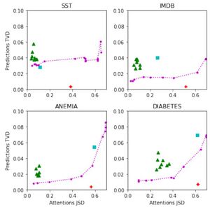  Figure 7: Averaged per-instance test set JSD and TVD from base model for each model variant. JSD is bounded at ~0.693. Green triangle: random seed; blue square: uniform weights; dotted line: the adversarial setup as $\lambda$ is varied; red plus: adversarial setup from Jain & Wallace (2019). Source: https://arxiv.org/abs/1908.04626

Table 3 presents the results. The first important result that the authors discuss is that, overall (across all datasets), using pre-trained LSTM attention weights is better than allowing the MLP to learn them on its own, which in turn is better than the unweighted baseline (uniform). Upon comparing these results with those in Table 2, the authors notice that this setup also outperforms the LSTM trained with uniform attention weights, which suggests that the attention module is more important than the word-level architecture for these datasets. The authors use these results to strengthen the case against the notion that attention weights are arbitrary. They further explain their position by stating that, as can be observed, independent token-level models that do not have access to contextual information still find attention weights useful, which indicates that they encode some measure of token importance that is not model dependent.

Training an adversary

Table 4: Best-performing adversarial models with instance-average JSD > 0.4. Source: https://arxiv.org/abs/1908.04626

The authors propose a model-consistent training protocol for finding adversarial attention distributions through a coherent parameterization which holds across all training instances.

Given a base model $M_{b}$, the authors train a model $M_{a}$ whose explicit goal is to provide similar prediction scores for each instance while attempting to have as different attention distributions from $M_{b}$ as possible. They train the adversarial model using stochastic gradient updates based on the following loss formula that is summed over instances in the minibatch: $L(M_{a},M_{b})^{(i)}=TVD({\hat {y}}_{a}^{(i)},{\hat {y}}_{b}^{(i)})\,-\,\lambda \,KL(\alpha _{a}^{(i)}||\alpha _{b}^{(i)})$ where ${\hat {y}}^{(i)}$ and $\alpha ^{(i)}$ denote predictions and attention distributions for an instance $i$, respectively. $\lambda$ is a hyperparameter that the authors use to control the tradeoff between relaxing the prediction distance requirement (low TVD) in favor of more divergent attention distributions (high TVD) and vice versa.

In Table 4, the authors present the highest F1 scores of models whose attention distributions diverge from the base by at least 0.4 in JSD (on average) along with their $\lambda$ setting and corresponding comparison metrics. They observe that all F1 scores are on par with the original model results reported in Table 2, signifying that the adversarial models are able to mimic the base model scores on the test sets. Next, the authors train a guided MLP model on these adversarially-trained attention distributions, the results of which are in the bottommost row of Table 3. The results show that although these adversarially-trained attention distributions have good local decision-imitation abilities, they are incapable of providing a non-contextual framework with useful guides. Using this results, the authors argue that even when the adversarial distributions are obtained consistently for a dataset, they deprive the underlying model from some form of understanding it gained over the data.

Additionally, the authors state that when the interaction between JSD and TVD is plotted on a two-dimensional axis, the shape of the plot can be interpreted to either support the "attention is not explanation" hypothesis (if it is convex i.e. JSD is easily maneuverable) or refute it if it is concave (early increase in JSD comes at a high cost in prediction precision). Hence, they present the plots in Figure 7 which show the levels of prediction variance (TVD) allowed by models achieving increased attention distance (JSD) on all four datasets. Although the convex shape of most curves may indicate that attention scores are easily influenced, the authors note that the extend of this effect in Jain & Wallace's (2019) per-instance setup is heavily exaggerated (i.e., the red cross on the plots is well below the curve).

Discussion and conclusions

Rudin (2018) defines explainability as simply a plausible (but not necessarily faithful) reconstruction of the decision-making process, and Riedl (2019) classifies explainable rationales as valuable in that they mimic what we as humans do when we rationalize past actions: we invent a story that plausibly justifies our actions, even if it is not an entirely accurate reconstruction of the neural processes that produced our behavior at the time. The authors, Wiegreffe & Pinter (2019), state that if they accept the Rudin (2018) and Riedl (2019) definitions of explainability as providing a plausible (but not necessarily faithful) rationale for model prediction, then the argument against attention mechanisms because they are not exclusive (as claimed by Jain & Wallace (2019)) is invalid. Just because another explanation exists doesn't mean that the one provided is false or meaningless, and the existence of multiple different explanations is not necessarily indicative of the quality of a single one. Additionally, Wiegreffe & Pinter (2019) show that alternate plausible explanations (from adversarial training methods) perform poorly relative to traditional attention mechanisms when used in the diagnostic MLP model (Table 3). This indicates that trained attention mechanisms in LSTMs on the selected datasets do learn something meaningful about the relationship between the inputs and outputs, and this relationship cannot be easily 'hacked' adversarially.

My thoughts on the contributions

What these works ultimately establish is that attention is not a silver bullet for interpretability and should not be relied upon as the sole explanation for a model's behavior. Attention should be seen as a tool, not a solution, and ideally should be combined with other techniques (such as saliency maps and layer-wise relevance propagation) to better understand the reasoning of the model. Additionally, when the interpretability of the model is crucial, one should use more interpretable models (such as linear models) (Rudin, 2018).

More specifically, this incremental work shows how ambiguous the criteria are for determining if a particular explanation is valid. Both works approach the notion of attention as an explanation method from two different perspectives; Jain & Wallace (2019) define attention and explanation as measuring the "responsibility" each input token has on the prediction (which is a more rigorous criteria to fulfil) whereas Wiegreffe & Pinter (2019) define attention and explanation as simply a plausible reconstruction of the model's decision making process. Determining which criteria are necessary and which are nice-to-have when it comes to determining if an explanation method is valid is still an active research subject in the field of XAI. Nonetheless, the authors' insights into the limitations of attention and the different assessments to determine the meaning behind these distributions is an extremely valuable contribution.

Annotated Bibliography

Put your annotated bibliography here. Add links where appropriate.

To Add

Put links and content here to be added. This does not need to be organized, and will not be graded as part of the page. If you find something that might be useful for a page, feel free to put it here.