Course:CPSC522/Analysis of hierarchical posterior for Language modeling

Analysis of hierarchical prior for language modeling

Principal Author: Kevin Dsouza
Collaborators:

Hypothesis

Implementing hierarchical prior ramps up the performance of the language model

Builds on

This page builds on

Introduction

To start off, let us first understand why we need to form hidden representation of our data. Given data $X$ (image or sentence), we want to express it in the form of hidden (latent) variables $Z$ through a network that can model the relationship between them. These hidden variables store the salient information of the given data. In the domain of Natural Language Processing, this compact representation can be utilized to do a variety of tasks such as classification, reconstruction, and translation. This relation between the data ( $X$ ) and the hidden variables ( $Z$ ) can be modeled by the posterior distribution $P(Z|X)$ . In case of sequential data, this distribution can be modeled by using recurrent neural frameworks like a Long Short-Term Memory (LSTM) or a Gated Recurrent Unit (GRU).

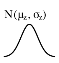
Figure 1: The hidden space used by a VAE

In a regular Recurrent Neural Network Language Model (RNNLM), the hidden representation is a deterministic vector (usually the hidden state of the LSTM) which forms the basis for future operations. The RNN is very good at mimicking the local statistics of the given data and naturally adapts to represent the statistics of the n-grams present in the data sequence. What is therefore lacking is variability in representation, which is a fundamental nature of generative models and human language itself. Here is where the variational models come in. Instead of a deterministic representation of the entire sequence, the variational models drive the representation to a space around this vector from which samples can be drawn later. Figure 1 shows such a Gaussian distribution whose mean ( $u_{z}$ ) and variance ( $\sigma _{z}$ ) are parametrized using a neural network.

In order to drive the hidden representation to a distribution, we need to have prior knowledge of the distribution that we want to be close to. This prior distribution of the latent variables P(Z) is usually chosen to be a Normal Gaussian. We want our posterior distribution to be as close to our prior distribution as possible (in the end) so that the samples that we draw later from the prior will be able to reconstruct the data distribution satisfactorily (Let us assume for the sake of explanation that our task is reconstruction of the original data distribution). How is it possible that a sample drawn from a normal Gaussian can regenerate the data distribution? The key here is to understand that any distribution in $d$ dimensions can be generated by a set of $d$ variables that are normally distributed via a mapping using a complicated function ^[1]. This complicated function in our case can be a neural network that learns useful latent representation at some layer and then uses this to further generate the data distribution (decoder).

Variational Autoencoders

Variational Autoencoders (VAEs) are a class of autoencoders that aim to reconstruct the data distribution by introducing variability in the intermediate representation. The joint distribution of $X,Z$ can be written as $P(X,Z)=P(X|Z)P(Z)$ , which requires you to draw a sample from the prior $P(Z)$ and and then sample from the conditional likelihood of $P(X|Z)$ . This $P(X|Z)$ can be any distribution like a Bernoulli or a Gaussian.

Now the inference in our model i.e. getting good latent variables conditioned on the data samples or the posterior $P(Z|X)$ is given by

Figure 2: Graphical Model describing a VAE

$P(Z|X)={\frac {P(X|Z)P(Z)}{P(X)}}$

The issue with this is that the real posterior is intractable as the denominator is a marginal written as

$P(X)=\int _{Z}P(X|Z)P(Z)\,dz$

which requires us to compute the integral over all the configuration of latent variables and is thus exponentially complex.

Therefore an approximate posterior $Q(Z|X)$ is designed to mimic the true posterior and a lower bound to the log marginal distribution is maximized as shown below.

We want to maximize the expectation of the log marginal distribution $P_{\theta }(X)$ under the given data distribution $P_{data}(X)$ . $P_{\theta }(X)$ is the actual distribution of the data whereas $P_{data}(X)$ is the one that we reconstruct. i.e.

$\max E_{X\sim P_{data}(X)}[log(P_{\theta }(X))]$

Now the log marginal is itself an expectation over the samples of latent variables ( $Z$ ) taken from the posterior ( $P_{\theta }(Z|X)$ because of the fact that we want to obtain hidden variables that can best explain the data.

$log(P_{\theta }(X))=E_{Z\sim P_{\theta }(Z|X)}[log(P_{\theta }(X)]$

From Bayes rule we have,

$P_{\theta }(X)={\frac {P_{\theta }(X,Z)}{P_{\theta }(Z|X)}}$

Putting this back in we get,

$E_{X\sim P_{data}(X)}[log(P_{\theta }(X))]=E_{X\sim P_{data}(X)}[E_{Z\sim P_{\theta }(Z|X)}[log({\frac {P_{\theta }(X,Z)}{P_{\theta }(Z|X)}})]]$

The issue with this is that the true posterior is intractable as it involves calculating the marginal by integrating out the all latent variables. Therefore an approximate posterior $Q(Z|X)$ is designed. This results in,

$=E_{X\sim P_{data}(X)}[E_{Z\sim Q_{\phi }(Z|X)}[log({\frac {P_{\theta }(X|Z)P_{\theta }(Z)}{P_{\theta }(Z|X)}})]]$

$=E_{X\sim P_{data}(X)}[E_{Z\sim Q_{\phi }(Z|X)}[log(P_{\theta }(X|Z)]-E_{Z\sim Q_{\phi }(Z|X)}[log({\frac {P_{\theta }(Z|X)}{P_{\theta }(Z)}})]]$

$=E_{X\sim P_{data}(X)}[E_{Z\sim Q_{\phi }(Z|X)}[log(P_{\theta }(X|Z)]-E_{Z\sim Q_{\phi }(Z|X)}[log({\frac {P_{\theta }(Z|X)}{P_{\theta }(Z)}}*{\frac {Q_{\phi }(Z|X)}{Q_{\phi }(Z|X)}})]]$

$=E_{X\sim P_{data}(X)}[E_{Z\sim Q_{\phi }(Z|X)}[log(P_{\theta }(X|Z)]-E_{Z\sim Q_{\phi }(Z|X)}[log({\frac {Q_{\phi }(Z|X)}{P_{\theta }(Z)}})]+E_{Z\sim Q_{\phi }(Z|X)}[log({\frac {Q_{\phi }(Z|X)}{P_{\theta }(Z|X)}})]]$

The second term is the KL divergence between the approximate posterior and the prior $KL(Q_{\phi }(Z|X)||P_{\theta }(Z))$ and the final term is the KL divergence between the approximate posterior and the true posterior $KL(Q_{\phi }(Z|X)||P_{\theta }(Z|X))$ .

Therefore we get,

$=E_{X\sim P_{data}(X)}[E_{Z\sim Q_{\phi }(Z|X)}[log(P_{\theta }(X|Z)]-KL(ApproxPost||Prior)+KL(ApproxPost||TruePost)]$

As the true posterior is intractable this cannot be directly estimated. But as the KL divergence is always positive, the third term can be taken to the left and thus lower bound is obtained. This lower bound is called the variational lower bound and forms the basis of optimizing the variational autoencoders.

$E_{X\sim P_{data}(X)}[[log(P_{\theta }(X))]-KL(ApproxPost||TruePost)]=E_{X\sim P_{data}(X)}[E_{Z\sim Q_{\phi }(Z|X)}[log(P_{\theta }(X|Z)]-KL(ApproxPost||Prior)]$

$E_{X\sim P_{data}(X)}[log(P_{\theta }(X))]\geq E_{X\sim P_{data}(X)}[E_{Z\sim Q_{\phi }(Z|X)}[log(P_{\theta }(X|Z)]-KL(ApproxPost||Prior)]$

The RHS is the variational lower bound which has to be maximized. When optimizing we minimize the negative of the lower bound. This can be broken down into two terms, the reconstruction loss (negative log likelihood of data) and the KL loss.

Figure 3: Hierarchical Posterior

Figure 2 shows the graphical model describing the VAE. The generative function is given by $P_{\theta }(X|Z)$ , where $\theta$ are the generative model parameters. The inference function is our approximate posterior given by $Q_{\phi }(Z|X)$ , where $\phi$ are the inference model parameters.

The question remains whether a single posterior distribution is informative enough to capture the nuances of a lengthy sentence. If the underlying data distribution is fairly complex (highly multimodal), then a regular posterior won’t do a good job of modeling the same. Therefore, it would seem natural for us to move to more complex posterior distributions that can be close to the real intractable posterior such that the variational lower bound is maximized. Towards this end, we can explore a hierarchical posterior distribution which can exploit the natural hierarchy that exists in a sentence. By this, I mean that each word is partly dependent on the word that precedes it and influences the word that follows it, and altogether these words become dependent in the context of the entire sentence. A posterior that can model these rich dependencies would allow the exploration of global sentence context.

Hierarchical Posterior

When the posterior is hierarchical, all the words are dependent on the words preceding them. Adding to this a global latent variable is considered that is dependent on all the words in the sentence in order to give the sentence context. This posterior can be written as

$q(z_{g},z_{w},x)=q(z_{g}|z_{w_{n}},z_{w_{n-1}},....,z_{w_{0}},X)*q(z_{w_{n}}|z_{w_{n-1}},....,z_{w_{0}},w_{n})*q(z_{w_{n-1}}|z_{w_{n-2}},....,z_{w_{0}},w_{n-1})......*q(z_{w_{0}}|w_{0})$

Figure 4: Reconstruction Loss

Figure 3 shows this dependence more clearly. It can be seen that every latent word sample ( $z_{x}$ ) depends on the previous latent word and the current word ( $w_{x}$ ). The global latent depends on all the latent words.

Hierarchical Prior

A hierarchical prior will look much like the for hierarchical posterior and has similar properties in the sense that it has richer representational power. This departure from normal Gaussian might help in modeling data that is highly multimodal in nature. The hierarchical prior can be written as

$p(z_{g},z_{w})=p(z_{g})*p(z_{w_{0}}|z_{g})*.....*p(z_{w_{n}}|z_{w_{n-1}},....z_{w_{0}},z_{g})$

Figure 5: KL Loss for the words

The prior is modeled in such a way that all the latent words depend on the latent words preceding them and the global latent. It should be noted that the global latent variable is considered to be a Normal Gaussian.

Figure 6: KL Loss for the global latent

It would intuitively make sense to argue that the prior we are assuming should be descriptive enough to represent the data. Would it be acceptable for the prior to be a simple (normal gaussian say) and the posterior to be hierarchical and complex? In which case will the posterior perform better? This is something that I plan to check using experiments and will draw conclusions from the results that I obtain.

Evaluation

The evaluation is conducted on the English Penn TreeBank dataset. Penn Treebank dataset is a large annotated corpus consisting of over 4.5 million words of American English ^[2]. All the models are run using the Deep Learning framework Tensorflow.

With hierarchical prior and hierarchical posterior

The first experiment I conduct is with a hierarchical prior, with only the global latent being a Normal Gaussian.

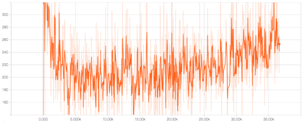
Figure 4 shows the reconstruction loss, which is the negative log likelihood of the data. It can be seen that the reconstruction loss decreases up to 5000 time steps after which there is a steady increase. This is because during training a concept called KL annealing is implemented. This involves zeroing the KL loss and gradually increasing its weight to 1. So until 5000 time steps, the network focuses entirely on reconstruction and hence the decrease. But later, the KL term kicks in we see the reconstruction suffering.

From Figure 5 we can see that the KL loss starts high and rapidly decreases. This is characteristic of a VAE where it tries to match the posterior with the prior and reduce the KL loss. In our case, we have two RNNs with high representational power mimicking the prior and the posterior, which might be the reason why they match up so soon. The KL loss for the global latent shows a similar behavior as seen in Figure 6.

With simple prior and hierarchical posterior

In this experiment, a Normal Gaussian prior is used for all the words and the global latent representation.

Conclusions

Annotated Bibliography

↑ A tutorial on Variational Autoencoders
↑ Marcus, Mitchell P., Mary Ann Marcinkiewicz, and Beatrice Santorini., 1993, "Building a large annotated corpus of English: The Penn Treebank.", Computational linguistics 19.2 (1993): 313-330.